Introduction
JETCARP, Jimmie’s Euclidean Tilings and Cellular Automata Research Program, runs cellular automata on almost any tiling of the plane: squares and hexagons, all eleven Archimedean tilings, the 1,248 k-uniform tilings up to k = 6, 81 isohedral tile types, tiles you draw yourself, and the aperiodic Penrose, hat and spectre tilings. It runs Life and the Life-like rules, Generations, Larger than Life, Langton’s ant and the turmites, WireWorld, the cyclic and excitable rules, sandpiles, Lenia and more, several at once if you like, on shared or separate fields. It is one program, with a graphical app, a command line, a scripting language and a Model Context Protocol (MCP) server for AI assistants, and it comes with tools that search for spaceships, oscillators and other patterns and keep verified catalogues of what they find.
This is version 0.4.0, the first public release; the changelog lists what it does, and How JETCARP was made tells where it came from.
Who it is for
- Desktop art. JETCARP can run a scene as a live wallpaper behind your windows, as a screensaver, or as still wallpapers cut to your monitors, in thirty built-in palettes or your own. Start with Your first live wallpaper.
- Hobby exploration. Pick an entry from Quick Start, move it to another tiling, change the rule, draw your own tile, and see what happens. Searching for your own spaceships takes one command. Start with Life on a new tiling.
- Research. Every run is a scene that replays bit for bit and records its state hash; every catalogued pattern has been verified exactly; the searches are resumable jobs whose results do not depend on the thread count and are designed not to depend on the machine; and everything can be scripted. Start with Core ideas and Reproducibility.
A gallery


JACA B27/S013); where the two signs meet, both are
destroyed. Scene docs/scenes/automata/jaca-hat-war.json. Right: James Edmond's
Spectre glider, two gliders crossing a tiling that never
repeats. Scene docs/scenes/automata/priority-spectre-glider.json.

docs/scenes/tilings/ship-57a0326c.json. Right: the
cyclic automaton organising noise into spirals on the hat. Scene
docs/scenes/automata/cyclic-hat.json.
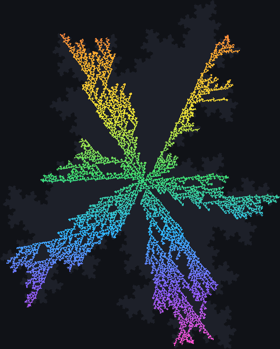
RNL on the trihexagonal
tiling, which builds a highway after about 2,600 steps of disorder. Scene
docs/scenes/automata/turmite-trihex-highway.json. Right: the
layered rule Layer 2/01 grown from one tile of the
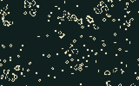
spectre tiling. Scene docs/scenes/automata/layered-spectre.json.Every picture in this book is made by JETCARP from the scene named under it, so you can run any of
them yourself: jetcarp run <scene> --gens N --png out.png.
Two ways through this book
- Desktop and hobby. Getting started, then tutorials 1 and 2, then the guides (for example Wallpapers and Searching for patterns) as you need them.
- Research. Getting started and Core ideas, then the encyclopedia of cellular automata and tilings, then Research (reproducibility, search methods, what is new, findings and the bibliography) and the Reference pages.
Standing on earlier work
Almost nothing in JETCARP’s rules and tilings is new: they are the work of many people over seventy years, credited on the page for each family and tiling, in the bibliography, and in Credits. The few things that, as far as we can tell, are new are listed with their evidence in What is new in JETCARP, together with what we decided not to claim. JETCARP was built with heavy use of an AI coding assistant; How JETCARP was made says how, and how its results were checked.
Where to go next
- Install JETCARP and set it up.
- Read the core ideas: tilings, cell fields, rules and scenes.
- See what is new and what the searches found.
- Cite JETCARP if it helps your work, and contribute if you would like to.
Installing JETCARP
JETCARP is one program, jetcarp: with no subcommand it opens the app, and its subcommands are the
command line, the background host and the MCP server. Every way of installing it below gives the
same program. Pick the one that suits the tools you already use:
| Way | Systems | Starter pack | Updates with |
|---|---|---|---|
| The installers | Linux, macOS, Windows | yes | running the installer again |
| pipx, uv or pip | Linux, macOS, Windows | yes | pipx upgrade jetcarp, uv tool upgrade jetcarp |
| Homebrew | macOS, Linux | yes | brew upgrade jetcarp |
| Scoop | Windows | yes | scoop update jetcarp |
| A release archive | Linux, macOS, Windows | yes | downloading the next one |
| cargo | anywhere Rust runs | no | cargo install jetcarp again |
Release builds are made for Linux on x86_64 and ARM (aarch64), Windows on x86_64, and macOS on Apple silicon and Intel. Linux on ARM and Intel Macs are built by the same release workflow but have not been tried by hand. On anything else, cargo builds JETCARP from source.
Before JETCARP’s repository is public. The commands on this page are written as they will be
for the 0.4.0 release. The release files, PyPI, crates.io, the Homebrew tap and the Scoop bucket
appear with it; until then the links here do not work. Release candidates such as 0.4.0-rc.1 are
published on GitHub only, for testing; see Release candidates.
The installers
On Linux and macOS, in a terminal:
curl -LsSf https://github.com/jprodgers/jetcarp/releases/latest/download/jetcarp-installer.sh | sh
On Windows, in PowerShell:
powershell -ExecutionPolicy Bypass -c "irm https://github.com/jprodgers/jetcarp/releases/latest/download/jetcarp-installer.ps1 | iex"
Each installer downloads the release archive for your computer and the release’s SHA256SUMS,
refuses the archive if its checksum does not match, and unpacks it into a folder of its own:
| Linux and macOS | Windows | |
|---|---|---|
| The program’s folder | ~/.local/lib/jetcarp | %LOCALAPPDATA%\Programs\jetcarp |
On your PATH as | a link, ~/.local/bin/jetcarp | the folder, added to your user PATH |
Nothing else is changed: no administrator rights are needed, no system folders are touched, and the
shell installer never edits your shell’s startup files. If ~/.local/bin is not on your PATH, it
says so and shows the line to add. On Windows, open a new terminal afterwards so that it sees the
new PATH.
The installers take options. With the shell installer, put them after sh -s -- (or download the
script and run sh jetcarp-installer.sh OPTIONS); with PowerShell, download
jetcarp-installer.ps1 and run it with the options, or set the environment variable named with
each before irm | iex.
| Shell | PowerShell | Variable | Does |
|---|---|---|---|
--version V | -Version V | JETCARP_VERSION | Install release V, such as 0.4.0 or 0.4.0-rc.1, instead of the installer’s own |
--no-packs | -NoPacks | JETCARP_NO_PACKS=1 | Leave out the starter pack |
--dir DIR | -InstallDir DIR | JETCARP_INSTALL_DIR | Install into another folder |
--bin-dir DIR | JETCARP_BIN_DIR | Put the link in another folder | |
-NoModifyPath | JETCARP_NO_MODIFY_PATH=1 | Leave the user PATH alone | |
--url URL | -DownloadUrl URL | JETCARP_DOWNLOAD_URL | Take the release files from another address, or from a folder that holds them |
--gh | -UseGh | JETCARP_USE_GH=1 | Download with the GitHub CLI, signed in, which can read a private repository |
--uninstall | -Uninstall | Remove what the installer installed |
An installer only ever replaces a folder it made itself (it leaves a .jetcarp-installer file
there), and refuses to replace a jetcarp on your PATH that something else put there, such as
pipx or cargo.
With pipx, uv or pip
JETCARP’s Python package contains the program and the starter pack, and no Python code. It installs
the program onto your PATH like any Python tool:
pipx install jetcarp
# or
uv tool install jetcarp
# or, inside a virtual environment
pip install jetcarp
The wheels are built for the same systems as the release archives, for any Python 3.8 or newer;
there is no source package, so on other systems use cargo. The starter pack goes in
share/jetcarp/packs inside the Python environment, and on macOS the screen saver’s code in
lib/jetcarp.
With Homebrew
On macOS or Linux:
brew tap jprodgers/jetcarp
brew install jetcarp
brew install jprodgers/jetcarp/jetcarp does both in one line. The formula installs the release
archive; nothing is compiled. The starter pack is in $(brew --prefix)/share/jetcarp/packs.
With Scoop
On Windows:
scoop bucket add jetcarp https://github.com/jprodgers/scoop-jetcarp
scoop install jetcarp
Scoop adds jetcarp to your PATH and a JETCARP entry to the Start menu, which starts the app
without a console window.
From a release archive
Each release on GitHub has an archive for each
system, such as jetcarp-0.4.0-x86_64-unknown-linux-gnu.tar.gz or
jetcarp-0.4.0-x86_64-pc-windows-msvc.zip. Unpack it anywhere and run jetcarp from the folder,
or put the folder on your PATH. The folder holds:
jetcarp(jetcarp.exeon Windows), the program;- on Windows
jetcarpw.exe, which starts JETCARP without a console window, for shortcuts and the screen saver; keep it besidejetcarp.exe; - on macOS
libjetcarp_saver.dylib, the screen saver’s code, whichjetcarp host saver installuses; keep it besidejetcarp; packs/, the starter pack;README.md, the licences (COPYING,UNLICENSE,LICENSE-MIT),THIRD_PARTY_NOTICES.mdandTHIRD_PARTY_LICENSES.html, the notices of the libraries the program is built from.
With cargo
With Rust 1.95 or newer and a C compiler (for the SQLite and Zstandard libraries JETCARP builds in), cargo builds JETCARP from source:
cargo install jetcarp
From a copy of the repository, cargo install --path crates/jetcarp --profile dist builds the same
way as the releases do: the dist profile leaves out debugging information, which would otherwise
make the program several hundred megabytes. cargo installs only the program, so there is no starter
pack (jetcarp paths says so); you can import packs yourself. On Linux the
build needs no system libraries: windowing, Wayland, X11 and Vulkan are all loaded when the program
runs.
Release candidates
Before a release, its candidates (0.4.0-rc.1, 0.4.0-rc.2 and so on) are published on GitHub as
pre-releases, for testing. They are not on PyPI, crates.io, Homebrew or Scoop, and they are never
GitHub’s “latest” release, so name the one you want. Use the installer attached to it:
curl -LsSf https://github.com/jprodgers/jetcarp/releases/download/v0.4.0-rc.1/jetcarp-installer.sh | sh
powershell -ExecutionPolicy Bypass -c "irm https://github.com/jprodgers/jetcarp/releases/download/v0.4.0-rc.1/jetcarp-installer.ps1 | iex"
or any installer with --version 0.4.0-rc.1 (-Version 0.4.0-rc.1 in PowerShell). Installing
the release itself later replaces the candidate.
On each system
Linux
The release builds run on Linux with glibc 2.28 or newer: Debian 10, Ubuntu 20.04, Fedora 29, RHEL, Rocky and AlmaLinux 8, and anything newer. They are not built for musl systems such as Alpine, where cargo works instead.
The command line needs nothing beyond glibc. The app, the background host and the GPU simulation load these libraries when they start, which a desktop system already has:
- a Vulkan driver (
libvulkan.so.1with Mesa’s or your graphics card’s driver), or failing that OpenGL ES through EGL (libEGL.so.1); - for windows,
libwayland-client.so.0on Wayland orlibX11.so.6,libX11-xcb.so.1,libxcb.so.1,libXcursor.so.1andlibXi.so.6on X11, andlibxkbcommon.so.0(withlibxkbcommon-x11.so.0on X11); - for the app’s file dialogs,
libdbus-1.so.3and an XDG desktop portal.
jetcarp doctor shows the graphics adapters it found; with none, simulation runs on the CPU.
macOS
The release builds run on macOS 11 (Big Sur) or newer. They are not signed with an Apple Developer ID, so the first time you open one that your browser downloaded, macOS says it cannot check it for malicious software and will not open it. Either remove the mark the browser left on the archive before unpacking it:
xattr -d com.apple.quarantine jetcarp-0.4.0-aarch64-apple-darwin.tar.gz
or, after the warning, open System Settings → Privacy & Security and click Open Anyway beside
the message about jetcarp. The installers, Homebrew, pipx, uv and pip download without that mark,
so this applies only to an archive downloaded in a browser. The screen saver bundle that
jetcarp host saver install makes is signed on your Mac, ad hoc, as macOS requires.
Windows
The release builds run on 64-bit Windows 10 and 11, and on Windows on ARM through its x64 emulation. They are not yet signed, so Windows SmartScreen may stop a program from a zip that your browser downloaded with Windows protected your PC. Click More info, then Run anyway; or, before unpacking, open the zip’s Properties and tick Unblock. The PowerShell installer and Scoop download without the browser’s mark, so this applies only to an archive downloaded in a browser.
jetcarpw.exe, beside jetcarp.exe, starts JETCARP without opening a console window; shortcuts, the
login entry and the screen saver use it.
The starter pack
Releases come with a starter pack: a folder of packs (each a pack store, as Pack format lays out) that the first-run setup offers to import into your library. JETCARP looks for this folder in one place, the first of:
JETCARP_BUNDLED_PACKS, if it is set;share/jetcarp/packsbeside the folder the program is in (<program folder>/../share/jetcarp/packs), where Homebrew and the Python package put it;packsin the program’s folder, as in the release archives and the installers’ folders.
The program’s folder is the one the program really is in: a link to it on your PATH, as pipx, uv,
Homebrew and the installers make, is followed. jetcarp paths shows the folder it found as
bundled:, and jetcarp doctor its size, or where it looked when there is none. JETCARP reads the
folder and never writes to it. To import a pack from it yourself, run jetcarp pack import with the
pack’s folder.
Checking a download
Each release has a SHA256SUMS file listing the SHA-256 of every file in it. The installers check
the archive they download against it; to check a file you downloaded yourself, put SHA256SUMS in
the same folder and run
sha256sum --check --ignore-missing SHA256SUMS                      # Linux
grep jetcarp-0.4.0-aarch64-apple-darwin.tar.gz SHA256SUMS | shasum -a 256 --check   # macOS
or, in PowerShell, compare (Get-FileHash jetcarp-0.4.0-x86_64-pc-windows-msvc.zip).Hash with the
file’s line in SHA256SUMS (the case of the letters does not matter). Once the repository is
public, each release file also has a signed record of the workflow run that built it, which the
GitHub CLI checks:
gh attestation verify jetcarp-0.4.0-x86_64-unknown-linux-gnu.tar.gz --repo jprodgers/jetcarp
No telemetry
JETCARP makes no network connections. It does not check for updates, report crashes or collect
statistics of any kind; it never sends anything anywhere. The only sockets it opens are on your own
computer, for the app’s AI control and the background host (see
SECURITY.md). Packs and other files
reach it only when you give them to it.
Uninstalling
Run jetcarp uninstall first, while the program is still there, to undo what JETCARP set up outside
its folders; then remove the program the way you installed it. Uninstalling
has the details.
First run and setup
This page is being written.
A tour of the app
This page is being written.
Core ideas: tilings, cell fields, rules, scenes
JETCARP has a handful of ideas that the rest of this book takes for granted. This page introduces them briefly, in the order they build on each other, and points to the pages that explain each one properly.
A tiling is a neighbour graph
A tiling covers the plane with tiles, with no gaps and no overlaps: squares, hexagons, mixtures of polygons, shapes you draw yourself, or the aperiodic Penrose, hat and spectre tilings, which never repeat. Each tile is a cell of the automaton.
What a rule needs to know about a tiling is only who is next to whom. JETCARP turns every tiling into a neighbour graph: one node per tile, linked to its neighbours, kept in clockwise order around each tile. There are two kinds of neighbour. Touch neighbours share an edge or just a corner; on squares these are the eight cells of the Moore neighbourhood that Conway’s Life uses. Edge neighbours share a stretch of edge; on squares, the four cells of the von Neumann neighbourhood.
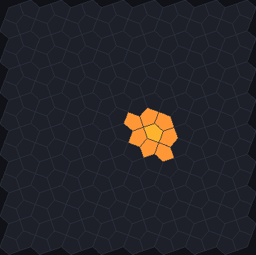
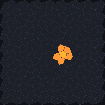
docs/scenes/automata/generalising-touch.json and
generalising-edge.json, 1 generation.On squares every cell has 8 touch neighbours. Elsewhere the numbers change, sometimes from tile to tile: a triangle touches 12 others, an octagon of the 4.8.8 tiling 8 and its squares 4, and a Penrose rhomb between 7 and 11. Most rules count neighbours, so the same rule behaves quite differently on different tilings, and that is much of what makes JETCARP interesting. Two tilings that look different can have the same graph, and then every counting rule behaves the same on both.
More: Tilings as neighbour graphs, How JETCARP generalises automata to any tiling, and the tiling catalogue.
Cells live in fields
The states of the cells are kept in a cell field: one value per tile. What a value means depends on the rule. A binary field holds live or dead cells, each with an age, the number of generations it has been in its state. A multi-state field holds a state number (Generations, WireWorld, turmite colours, JACA’s +1 and −1). A height field holds sandpile grains, and a continuous field holds a value between 0 and 1 (Lenia). Time moves in generations: every cell’s next state is computed from the current states of itself and its neighbours, all at once.
Rules and families
A rule says how a cell’s next state follows from its own state and its neighbours’. Rules come in
families, each with its own notation: Life-like rules written as
birth and survival counts (B3/S23 is Life), Generations rules with dying states (B2/S/C3), Larger
than Life with a larger range, Langton’s ant and the turmites, which are agents that walk and turn
(Ant RL), the cyclic and excitable rules, sandpiles, Lenia, priority tables, rule tables, and others.
Two families are, to our knowledge, new in JETCARP, both Jimmie Rodgers’s:
JACA, an annihilating two-sided Life, and layered rules,
which grow Wolfram-style row rules outward from a seed on any tiling (see
What is new in JETCARP). Many rules also have names, such as Life, HighLife or
Brian’s Brain.
Every family is written in terms of the neighbour graph, so almost every rule runs on almost every tiling. The few that are tied to a particular grid, such as the elementary row rules and von Neumann’s 29-state automaton, say so.
More: the encyclopedia of cellular automata, one page per family, and the named rule catalogue.
Several automata on one tiling
A world is one tiling with one or more automata on it, each with its own rule, seed and palette. Every generation the automata step in order. Automata of the same kind (all binary, say) share one field by default, so they act on each other’s cells: in the built-in scene Rule 30 meets Life and ants, Rule 30 writes rows, Life rewrites what it leaves behind, and three ants wander through both. An automaton with Affects others switched off keeps a private field instead, drawn alongside the others but untouched by them. Automata whose fields cannot be shared, such as a sandpile, always keep their own. A scene can also carry a script, which switches automata on and off in turn as conditions are met.
More: Several automata at once.
Scenes are how runs are kept
A scene is a small JSON file that holds everything needed to reproduce a run: the tiling, the
automata with their rules and seeds, the state of the random-number generator, and the log of every
change made since. Opening a scene replays it, so it comes back exactly as it was. A saved scene
records the generation and state hash it reached, and jetcarp verify checks that it still gets
there: the same scene gives the same state, bit for bit, on any number of threads, on the CPU or the
GPU, and, by design, on any operating system. Scenes are what you save and share, what the command line runs, and
what every picture in this book is made from.
More: Scenes: saving, sharing, reproducing, the scene file format and Reproducibility.
Quick Start
Quick Start is the menu of ready-made scenes that the app opens with, each shown as a live preview. Its entries come from four sources, all kept in the pattern library: the classics built into JETCARP (hand-made scenes and a working example of every named rule, each on the grid it is usually shown on), entries from the packs you import, the atlas of runs picked from an exploratory search, and My finds, the entries you add yourself from patterns, runs and scenes. It is the quickest way to see what JETCARP can do, and an entry, once open, is a scene like any other: move it to another tiling, change its rule, save it. Right-click a card to rate it or hide it.
More: A tour of the app and Building your own Quick Start.
The pattern library
The pattern library, or catalogue, is a database of verified patterns: still lifes, oscillators, spaceships and the like, each with the tiling it lives on and the range of rules it works in, plus the runs of ants and turmites and the record of every search. Nothing goes in unverified: each pattern is run again on its own and checked cell by cell before it is stored. Patterns can be pasted into a world, rendered as pictures and animations, and promoted to Quick Start.
More: The pattern library.
Jobs
Searches can run for minutes or for weeks, so each one runs as a job: a record in the catalogue with
the search’s settings, its progress and a checkpoint. A job can be stopped, closed with the program
and carried on later, on this machine, and it ends exactly as an uninterrupted run would. The command
line starts searches with jetcarp search <strategy> (soup hunts, ant searches, rule censuses, the
evolutionary glider search and others) and manages them with jetcarp jobs.
More: Searching for patterns and Search methods.
Your first live wallpaper
This page is being written.
Life on a new tiling
This page is being written.
Hunting for spaceships
This page is being written.
Building your own Quick Start
This page is being written.
5. Scripting a rule sweep
In this tutorial you write a short Rhai script that runs 64 cellular automaton rules on the Cairo pentagon tiling, one world per rule, in parallel on every core. Then you read the results back, lay your favourites out on a contact sheet, and put the best one in your Quick Start menu. It takes about fifteen minutes, and the sweep itself runs in a couple of seconds.
You need JETCARP installed (Installing) and a text editor.
Everything here runs from a terminal; the same scripts also run in the app, under
Tools → Scripts and sweeps…. Everything the scripts write goes into JETCARP’s output folder,
<Pictures>/JETCARP (see Folders).
1. One world
Start with a single world, to see what a script looks like. Save this as first.rhai:
// Life on Cairo pentagons: run 300 generations and save a picture and a scene.
let w = world(#{ tiling: "cairo", size: "120x80" });
w.add_ca("B3/S23", #{ seed: "random:0.35" });
w.step(300);
out_dir("cairo-life");
w.save_png("cairo-life.png");
w.save_scene("cairo-life.json");
print(`generation ${w.generation()}, ${w.population()} live cells, hash ${w.hash()}`);
and run it:
$ jetcarp script first.rhai
generation 300, 1527 live cells, hash 8c936c690b20f095
output: /home/ada/Pictures/JETCARP/2026-11-11_21-27-33_cairo-life
time:   0.10s
Line by line:
world(…)makes a world: here 120 × 80 unit cells of the Cairo tiling, with dead edges.add_caadds a cellular automaton to it, Conway’s Life (B3/S23), seeded with 35% of its cells alive.step(300)runs 300 generations.out_dir("cairo-life")makes a new folder in the output folder, named with the time and the label, and later file names are relative to it.save_pngandsave_scenewrite a picture and a scene.
Your hash will be the same as the one above: the same tiling, rules and seeds always give the same
world, on any computer and at any thread count. jetcarp verify cairo-life.json replays the scene
and checks that it reaches that hash again.
2. Sweep 64 rules
A sweep runs one world per rule. Instead of Life, take a random sample of 64 rules from a family:
births on 2 to 4 live neighbours, survival on 1 to 5, and four states. In a four-state
Generations rule, a dying cell fades through two more states before it is empty, which leaves
coloured trails behind anything that moves. Save this as sweep.rhai:
let s = sweep(#{
    rules: "B/S", birth: "2-4", survive: "1-5", states: 4,
    sample: 64, sample_seed: 1,
    tiling: "cairo", size: "64x40",
    seed: "random:0.35", rng_seed: 1,
    max_gens: 300, palette: "Prism",
    png: #{ size: [480, 300] },
    skip: ["empty", "full"],
    out: "cairo-gen",
});
print(`${s.runs} runs, ${s.images} pictures`);
$ jetcarp script sweep.rhai
sweep done: 64 of 64 runs, 50 images, 50 kept, 0 errors in 1.4s
64 runs, 50 pictures
output: /home/ada/Pictures/JETCARP/2026-11-11_21-29-35_cairo-gen
time:   1.37s
What the options do:
rules: "B/S"withbirthandsurvivedescribes every rule whose births and survivals fall in those ranges.sample: 64picks 64 of them at random, andsample_seedmakes it the same 64 every time.tiling,size,seedandrng_seedare the same for every run, so the rule is the only difference between them.max_gens: 300runs each world 300 generations;untilcan stop a run earlier, for instance when it stops changing.pngsets each picture’s size, andpaletteits colours.skip: ["empty", "full"]doesn’t save pictures of runs that died out or filled up, which is why 50 of the 64 runs have one.
The sweep’s folder holds a picture per run (03_B23_S1_C4.png and so on) and a manifest, as
manifest.csv and manifest.json, with a row per run: its rule, picture, final hash, population,
density, period if it settled into one, and, for rules that write row by row, a description of
its rows (row_class, row_hint). run.json records how the sweep was made.
Open the folder and look through the pictures. Some rules die at once, some freeze into specks, some crawl with worms, some boil.
3. Read the results back
The manifest is what makes a sweep useful beyond its pictures. manifest(folder) gives a script
its rows, so a second script can sort and filter them. Save this as pick.rhai:
// The runs still busy at the end, most cells alive first.
let rows = manifest(params.folder).filter(|r| r.kept && r.period == ());
rows.sort(|a, b| b.population - a.population);
for r in rows {
    print(`#${r.index}  ${r.rule}  ${r.population} cells`);
}
and give it the sweep’s folder with --set:
$ jetcarp script pick.rhai --set folder=/home/ada/Pictures/JETCARP/2026-11-11_21-29-35_cairo-gen
#53  B234/S1234/C4  7581 cells
#7  B24/S234/C4  7116 cells
#58  B23/S134/C4  7095 cells
…
--set key=value puts values in the map params. A run that never settled has no period, which
Rhai writes as (). Every row has the manifest’s columns, so you can sort by density, keep only
row_class == "periodic", and so on.
Measure more as you go. A sweep can also call a function of yours on every world when its run ends, and add what it returns to the manifest. Add this option to the sweep above to count each run’s still lifes and oscillators:
    keep: |w, n| {
        let o = w.objects();
        #{ still_lifes: o.totals.still_life, oscillators: o.totals.oscillator }
    },
and the manifest gains still_lifes and oscillators columns. Running the sweep again with the same
folder (folder: "…" instead of out:) reuses the runs already done. Since this changes what each
run records, start a new folder instead.
4. A contact sheet of your favourites
jetcarp sheet lays chosen runs out on one picture, each labelled with its index and rule:
$ jetcarp sheet --folder /home/ada/Pictures/JETCARP/2026-11-11_21-29-35_cairo-gen \
    --runs "#1,#2,#3,#4,#7" --cols 5 --thumb 240 --png favourites.png
sheet: favourites.png (1248x194)
Runs are named by their index in the manifest (#3), by their rule text ("B23/S1/C4"), or for a
numbered family by their number (n=588).
5. Keep the best one
When a run is worth coming back to, put it in your Quick Start menu:
$ jetcarp library promote-run /home/ada/Pictures/JETCARP/2026-11-11_21-29-35_cairo-gen "#3" --title "Cairo worms"
promoted: B23/S1/C4 as "Cairo worms" (run #3)
The entry holds the run’s tiling, rule and starting state, so opening it from the Quick Start menu
replays the run exactly as the sweep ran it. The run is also starred in the folder’s
favourites.json. A script can do the same with library().promote_run(folder, "#3").
Where to go from here
- Bigger sweeps. A sweep runs on every core and can be stopped with Ctrl-C: it saves its
manifest first and prints the command that carries it on. Rerunning it with
folder:set to its folder skips the runs already done. The named families"W","HexW","HexW3","HexT"and"HexT3 sum"are numbered, sorules: "HexW3", from: 0, to: 19682sweeps all 19,683 ternary hexagon rules. The example scripts that ship with JETCARP (Examples in the app’s script editor, and thecrates/jetcarp-script/scriptsfolder of the source repository) include sweeps of every elementary rule. - Without writing code. The app’s Sweep builder tab, under Tools → Scripts and sweeps…, builds the same sweeps from a form, and Sweep this world sweeps a rule over whatever world is open.
- More functions. Scripting lists every function: worlds, runs, objects, pictures, the pattern library, searches and large sandpiles.
Driving JETCARP from an AI assistant (MCP)
This page is being written.
Scenes: saving, sharing, reproducing
A scene is a small JSON file that holds everything needed to reproduce a run: the tiling, the automata with their rules and seeds, the starting state of the random-number generator, and the log of every change made since. Opening a scene replays that log, so the world comes back exactly as it was. A saved scene also records the generation and the state hash it reached, so anyone can check that it still gets there. This guide covers saving and opening scenes in the app, running and checking them from the command line, sharing them, and getting a scene back out of a picture. The file itself is described in Scene file format.
Save and open a scene in the app
- File → Save scene… (Ctrl+S) writes the current world as a scene. The file holds the tiling, the automata, the random state and every change since the last reset or change of tiling (the Command log pane lists them), together with the view (where the camera is, the zoom and the speed) and a record of the generation and state hash. The Scene pane confirms it with the file’s path and the hash.
- File → Open scene… (Ctrl+O) opens one. The world is rebuilt and its log replayed, so it opens at
the saved generation and in the saved view. You can also open a scene when the app starts:
jetcarp --scene scene.json. - Quick Start entries are scenes. Open one, change what you like, and save it.
Everything you do to a world goes into its log: painting cells, pasting library patterns, adding and
changing automata, reseeding, editing palettes, running. Consecutive runs are merged into one step
entry, so a long session does not make a long file. Edit → Reset, choosing another tiling, and a
new random state start the log again from a new base.
The state hash is shown at the right end of the menu bar, after the generation: hash 1adf6e32, the
first eight of its sixteen digits. Click it, or use Edit → Copy state hash, to copy the whole hash.
Worlds of more than about a million cells compute the hash only while paused, and show hash …
while they run.
Run a scene from the command line
jetcarp run loads a scene, replays its log, runs more generations if asked, and reports where it
ended:
$ jetcarp run crates/jetcarp-core/data/scenes/rule30-life-ants.json --gens 100 --png out.png --save out.json
scene:      crates/jetcarp-core/data/scenes/rule30-life-ants.json
tiling:     Square (parallelogram) (square): 38400 cells, 240x160 unit cells, 1 tile type(s), storage dense, edges dead
backend:    cpu (32 threads)
generation: 100
hash:       1adf6e3234b7f199
status:     Running
done:       no
field 0:    shared binary, 2124 live: Rule 30 [W30], Life [B3/S23], Langton's ant [Ant RL]
png:        out.png (1600x1067)
saved:      out.json
time:       0.03s on 32 threads
--gens N counts from where the scene ends: run out.json (saved at generation 100) with
--gens 50 and it stops at generation 150. The other options:
| Option | Effect |
|---|---|
--png FILE | A picture of the final state, with the scene and hash inside it (see below) |
--max-side N, --scale S | The picture’s longest side in pixels (default 1600), or its scale in pixels per world unit (a tile edge is about one unit) |
--save FILE | The resulting scene, with its generation and hash recorded |
--threads N | Worker threads (default: all cores); the hash does not depend on it |
--expect HASH | Fail unless the run ends on this hash |
--gpu | Run the generations on the GPU where the rules allow it; the result is identical |
--reseed, --reseed-now | Automatic reseed policies, or one reseed before running (see Reseeding) |
--json | The report as JSON |
Check that a scene still reproduces
jetcarp verify replays a saved scene and compares the generation and hash it reaches with the ones
it recorded:
$ jetcarp verify out.json
ok: generation 100 hash 1adf6e3234b7f199
If they differ it says so and exits with status 1:
Error: MISMATCH: recorded gen 100 hash 1adf6e3234b7f198, replayed gen 100 hash 1adf6e3234b7f199
A scene with no record, such as one written by hand, cannot be verified (scene has no recorded
hash); run it with jetcarp run --save to record one. For a check inside a script or a test, use
jetcarp run scene.json --gens N --expect HASH, which fails with hash mismatch: expected …, got …
unless the run ends on that hash. jetcarp verify always replays on the CPU, so it is also the way to
check a run made with --gpu.
The state hash
The state hash is a 64-bit number, printed as sixteen hexadecimal digits, computed from everything that decides what the world does next: every cell’s state and age, sandpile heights, Lenia’s values, the generation, the ants, and the progress of any script or reseed policy. Two worlds with the same hash are, in practice, in the same state. The hash does not depend on the number of threads or on whether the CPU or the GPU did the work, and by design it does not depend on the operating system.
One case needs care: a HashLife jump reaches exactly the same cells as stepping, but restarts every
live cell’s age at 1, so its state hash differs. Compare the hash of the cell states alone instead
(states_hash() in scripts, cells_hash in the world status that MCP tools read). How the hash is
computed and tested is in Reproducibility.
Share a scene
A scene is one text file, and it carries everything it needs: the rule tables and palettes it uses,
and the cells of any library pattern pasted into it, so it does not need your pattern library. Send
the file; the other person opens it in the app or runs jetcarp verify on it to confirm that their
machine reaches the same hash. Scenes work well in version control, and with the output of
jetcarp doctor they make a complete bug report.
A few limits apply:
- A scene names its format (now 1). A JETCARP that only knows an older format refuses a newer scene rather than guessing.
- Until JETCARP 1.0, a release may change how a rule or a tiling behaves. Such changes are deliberate and listed in the changelog, but an old scene may then reach a different hash. The Penrose rhombs already lay out their tiles differently from those of CART, JETCARP’s predecessor.
- Palettes you made travel inside the scene. A scene that names a palette the other person’s JETCARP does not know (a built-in palette added in a later release, say) still opens, drawn in Ember, with a warning; the name is kept, so saving the scene again keeps it.
Get the scene back from a picture
Every PNG made by jetcarp run --png, File → Export PNG…, File → Export wallpaper…,
jetcarp wallpaper, jetcarp hashlife --png and a script’s save_png carries its scene inside it,
as PNG text chunks: jetcarp:scene (the whole scene), jetcarp:version, jetcarp:generation,
jetcarp:hash and jetcarp:dead_boundary. A picture can therefore always be traced back to the run
that made it. (Animations and frames from jetcarp media do not carry them.)
JETCARP does not yet open a scene from a PNG itself, but any program that reads PNG text chunks can take it out. With Python and the Pillow library:
from PIL import Image
open("scene.json", "w").write(Image.open("out.png").text["jetcarp:scene"])
$ jetcarp verify scene.json
ok: generation 100 hash 1adf6e3234b7f199
Scenes everywhere else
- Scripts read and write scenes with
load_scene(path),scene_world(json),w.save_scene(path)andw.scene()(see Scripting (Rhai) API). - MCP tools have
load_sceneandget_scene(see MCP tools). - Pictures and the desktop.
jetcarp wallpaper scene.json,jetcarp media render --scene, screensaver profiles and rotations all take scene files (see Pictures and animations and Wallpapers, screensavers and the background host). - This book. Every figure is made from a scene, named under it, and for the still pictures
jetcarp run <scene> --gens N --png out.pngmakes it again.
To write a scene by hand, start from the short example in Scene file format; anything you leave out takes its default.
Several automata at once
A world can run any number of automata on one tiling, each with its own rule, seed, palette and settings. Every generation they step in turn. Whether they act on each other depends on their fields, the arrays of cell values they work on: automata of the same kind share one field by default, so each reads and writes the others’ cells; an automaton with Affects others switched off keeps a private field instead, drawn alongside the rest but untouched by them. This guide explains which automata share, how to change it, in what order they step, and how several fields are drawn.
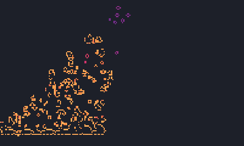
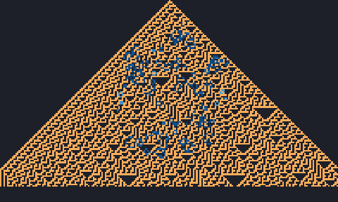
docs/scenes/guides/several-shared.json.
Right: with Affects others off for Life, it runs from a soup of its own on a private field,
drawn in blue over Rule 30's untouched triangle. Scene
docs/scenes/guides/several-separate.json.Which automata share a field
Every rule needs a certain kind of field:
| Field | Rules |
|---|---|
| Binary (live or dead, with ages) | Life-like rules, two-state Larger than Life, elementary rules, two-state hexagonal row and layered rules, Margolus rules, and ants and turmites with two colours |
| Multi-state (a state number, with a given number of states) | Generations, cyclic, Greenberg–Hastings, rock-paper-scissors, Hodgepodge, forest fire, WireWorld, JACA, the Spectre glider and other priority tables, rule tables, von Neumann’s automaton, and turmites with more than two colours |
| Height | The sandpile |
| Continuous (a value between 0 and 1) | Lenia |
- Binary rules share by default. Affects others starts on, and every binary automaton with it on works on the same field.
- Other rules start on a private field. Affects others starts off. Switch it on and the automaton
shares a field with the others of exactly its kind: the same field kind and the same number of
states. Two
B2/S/C3automata can share; aC3and aC4cannot. - Sandpiles never share. Their field holds grain heights, which no other rule understands, so the checkbox is greyed out.
When an automaton joins a shared field, its live cells are copied into it. When it leaves, it takes a private copy of the shared field as it is at that moment, and from then on the two evolve separately. A B/S rule added to a shared field that already has live cells, with no seed of its own, starts from those cells rather than scattering a random soup over another automaton’s work.
Order within a generation
The automata step in list order: the order they were added, or in a scene the order of its cas
list. Each takes its steps per generation (1 to 100,000) before the next begins, so on a shared
field a later automaton sees what an earlier one did in the same generation. Ants are usually given
many steps per generation (100 or 200 in the built-in scenes) so that they keep up with the cellular
automata around them. An automaton whose checkbox is cleared does not step at all, but its field
stays and is still drawn.
To have automata take turns over longer stretches, a scene can carry a sequence: a list of steps, each naming the automata that run during it and a trigger that moves on to the next (after a number of generations, when the population passes a value, when activity drops, when the world repeats, and so on). The Sequence pane builds one with New sequence, and Apply and start runs it; it is saved with the scene. The built-in Script: Rule 30, Day & Night, Seeds, Life, ants is a five-step example, and the format is in Scene file format.
In the app
- Add automata with CA → Add from catalog (the named rules, by family), CA → Add by notation…
(which opens the Add pane: pick a named rule and press Add, or type any rule in
notation such as
B36/S23orAnt RLR), or CA → Load rule table…. - The CAs pane has one card per automaton. Its header has the checkbox that runs it, its name and notation, and Remove. Inside are the rule, the neighbourhood (Touching or Edge), the Affects others checkbox with the field it is on (for example field 0 · shared binary · 3 CAs), Steps per generation, Colour by, Palette, and the Seed, Random and Clear buttons. Ant cards add + Ant and what ants do at a dead edge (Edge: bounce or Edge: fall off).
- Seed and clear every automaton at once from the Seed menu (Seed every CA, Random cells in every CA, Clear every CA), or one at a time from Seed → Each CA.
- Draw into one field. The Draw pane’s Into list chooses which automaton’s field the mouse paints.
From the command line, scripts and scenes
In a scene, affects_others is a field of each automaton:
"cas": [
  {"rule": "W30", "seed": "top_center"},
  {"rule": "B3/S23", "affects_others": false, "seed": {"blob": {"radius": 0.45, "density": 0.35}}}
]
In a script, it is an option of add_ca and update_ca:
let w = world(#{ tiling: "square", size: [200, 120], boundary: "dead" });
let r30 = w.add_ca("W30", #{ seed: "top_center" });
let life = w.add_ca("B3/S23", #{ affects_others: false, seed: "blob:0.45:0.35" });
w.step(110);
w.update_ca(life, #{ affects_others: true });   // join Rule 30's field from here on
jetcarp run reports every field and who is on it:
field 0:    shared binary, 6287 live: Rule 30 [W30]
field 1:    private binary, 584 live: Life [B3/S23]
How several fields are drawn
Each field is coloured by the first automaton in the list that uses it, with that automaton’s palette and Colour by setting. Changing the palette of a later automaton on a shared field therefore changes nothing you can see; change the first one’s. Fields are drawn in list order, later ones over earlier ones, with ants on top. Empty cells take the background of the first automaton’s palette, and the area outside the tiling its stage colour. The details are in Palettes.
Examples to try
- Rule 30 meets Life and ants (Quick Start): Rule 30 writes rows, Life rewrites what it leaves behind, and three ants taking 100 steps per generation wander through both, all on one binary field.
- Script: Rule 30, Day & Night, Seeds, Life, ants (Quick Start): five rules on one shared field, switched on one after another by a sequence.
- The two scenes of the figure above: run them with
jetcarp run docs/scenes/guides/several-separate.json --gens 110 --png out.png, then switch Affects others on and off in the app and watch the triangle.
More: Core ideas and How JETCARP generalises automata to any tiling.
Drawing and editing tiles
Many of JETCARP’s tilings can be reshaped, and new ones can be drawn from scratch. There are three tools: the tile editor, which bends the edges and moves the corners of a tile from one of the editable tile families or the isohedral types; the isohedral picker, which chooses one of Kaplan’s 81 isohedral types and sets its shape with sliders; and the unit cell editor, which draws any repeating arrangement of polygons. Whatever you make is saved in the scene, so a reshaped world replays exactly. (To paint cells rather than tiles, use the Draw pane.)
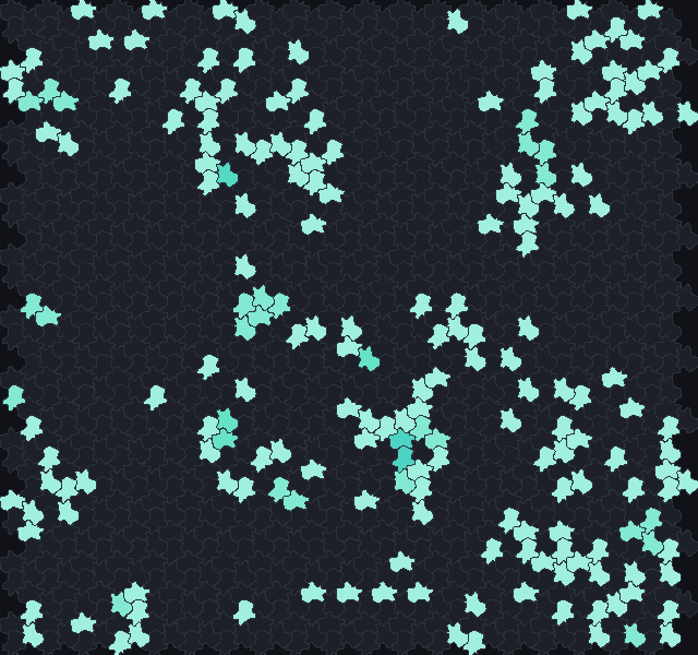
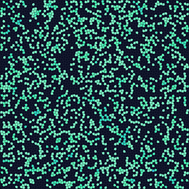
B2/S34. Scene docs/scenes/tilings/editable-lizard.json. Right: isohedral
type IH28 with Tactile's default shape. Scene docs/scenes/tilings/isohedral-ih28.json.What can be edited
| Tilings | Tile editor | Unit cell editor |
|---|---|---|
Editable families: lizard, hex, brick, square, quad, triangle, glide, fourfold, cairo | Corners and edges | Can start from one, with straight edges |
Isohedral types ih01 to ih93 (81 types) | Shape sliders and edges | Can start from one |
| Fixed tilings: the Archimedean tilings, the k-uniform catalogue, herringbone, Pythagorean squares, flat-topped hexagons | Fixed shapes | Can start from one and change it |
| Aperiodic: Penrose, hat, spectre | Fixed shapes | Not available |
For the editable families and the isohedral types, reshaping changes how a world looks, not how a rule behaves: the automata use the neighbour graph of the family, and dragging corners or bending edges does not change which tiles meet. When curved edges would make different tiles touch, the tile editor says for how many tiles, and that CAs use the straight-edge graph. In the unit cell editor, on the other hand, which tiles are neighbours is measured from the polygons you draw, so a new cell is a new graph.
The tile editor
Open it with Tiling → Tile editor…, or Edit tile… in the Tiling pane. The window shows the tile in the middle of a canvas, with ghost copies of its neighbours around it, and the controls on the right.
- Choose the family in the list at the top (the current tiling’s is chosen already). Below it are a note on the family and its symmetry group. For an isohedral type the type picker and its sliders appear here too (see below).
- Pick an edge. Edges come in colour-coded classes, and each edge’s partner follows it, so the tiles always fit. Click an edge to select its class (Edge class 2 of 3).
- Choose its shape: Free (any shape, which its partner copies), Mirror (symmetric about its midpoint), Half-turn (the same after a half turn) or Straight. Some choices are greyed out where the way an edge pairs with its partner allows only certain shapes, and the editor says so (This edge must stay half-turn symmetric to fit its neighbour).
- Bend it. Add point, or double-click an edge, adds a point; drag points and corners with the mouse; Delete point removes the selected one. Lines joins the points with straight segments, Curves with smooth curves.
- Use it. Use this tile rebuilds the world on the new tile. With Live ticked, the world is rebuilt after every edit.
Snap (Off, Square, Triangle) keeps points on a grid. Undo steps back, Randomize gives random edge shapes within the family’s rules, and Reset returns to the family’s default tile. A line under the controls says Valid tile, or Edges cross: tiles would overlap when an edge has been bent through another.
Copy tile JSON puts the tile on the clipboard as text, and Load JSON below reads one pasted into the box underneath, which is a way to keep and share tiles. (The Tiling pane’s Paste tile JSON from the prototype section reads tiles copied from JETCARP’s original JavaScript tiling editor.)
Isohedral types
In the Tiling pane’s family list, choose Isohedral IH01–IH93 (81 types). The type picker appears
under it: < and > step through the types, and the list shows each one’s symmetry group, number of
corners and number of parameters (for example IH28 p4 5 corners, 2 params). Each parameter has a
slider (p1 to p6; the world is rebuilt when you let go), and Default shape returns to Tactile’s
own. Types with no parameters say No shape parameters: the corners are fixed. Edges can still be
reshaped. To reshape the edges, open the tile editor, which shows the same picker; its edge choices
follow Tactile’s rules for the type, so the tile stays in it.
From the command line, jetcarp isohedral lists the 81 types with their symmetry groups and neighbour
counts, and jetcarp isohedral --png sheet.png draws all of them on one contact sheet (with random
edge shapes, or straight ones with --straight; --seed picks other random shapes). In a scene or a
script, a type and its parameters look like this:
"tiling": {"family": "ih28", "params": {"p": [0.45, 0.5]}, "size": {"cells": 2000}}
let w = world(#{ tiling: "ih28", params: #{ p: [0.45, 0.5] }, size: 2000 });
The unit cell editor
The unit cell editor draws tilings of the periodic family: two lattice vectors, which say how the
cell repeats, and any polygons inside one cell. Tiles may have different shapes and need not meet
edge to edge. Open it with Tiling → Unit cell editor…, or Edit unit cell… in the Tiling pane
(it is not available for the aperiodic tilings, which have no unit cell).
- Start from an empty square or hexagonal lattice, any fixed tiling, any tiling of the catalogue, or an editable family with straight edges.
- Tools. Select drags corners, whole tiles and the two lattice arrows; double-click an edge to add a corner. Draw tile adds a tile corner by corner: click the corners, then click the first one again, double-click or press Enter to close it; right-click removes the last corner and Esc cancels. Stamp n-gon puts a regular polygon with a chosen number of Sides on the edge you click (or in empty space), with options for its side length and which side of the edge it goes.
- Snapping. Snap to Corners, Edges and Angles, a Grid (Off, Square, Triangle), and Move shared corners together, so that dragging a corner drags every corner sitting on it. Ghost rings sets how many rings of neighbouring cells (1 to 3) are drawn around the cell.
- The selected tile can be deleted, duplicated or moved back into the cell, and its corners inserted or deleted. Undo, Redo and Fit view work as usual; scroll to zoom and drag empty space (or use the right button) to pan.
As you work, the editor checks the cell for overlaps between tiles and their copies, gaps, tiles that cross themselves and edges with nothing on the other side. It lists every tile with its number of corners, area and measured neighbours (by edge and touching), and says Valid tiling when all is well. Use this cell (available once there are no errors) rebuilds the world on it, and Live does so after every valid edit. Copy cell JSON and Load JSON below copy and paste the cell as text.
A cell in a scene or a script is written as the lattice vectors a1 and a2 and a list of polygons,
each a list of corners. This one cuts the unit square into two triangles:
"tiling": {"family": "periodic",
           "params": {"a1": [1, 0], "a2": [0, 1],
                      "polys": [[[0, 0], [1, 0], [1, 1]], [[0, 0], [1, 1], [0, 1]]]},
           "size": {"rect": {"w": 40, "h": 30}}, "boundary": "wrap"}
let cell = #{ a1: [1, 0], a2: [0, 1],
             polys: [[[0, 0], [1, 0], [1, 1]], [[0, 0], [1, 1], [0, 1]]] };
let w = world(#{ tiling: "periodic", params: cell, size: [40, 30], boundary: "wrap" });
In the scene
A reshaped or drawn tile is part of the scene’s tiling: its shape parameters in params and, for
tiles made in the tile editor, the shape of each edge in edges (see
Scene file format). Changing the tile starts the
world’s command log again from the new tiling, as any change of tiling does. Saved, the scene replays
to the same hash. JETCARP’s tests pin the geometry of every family’s default shape and
every catalogued tiling; a tile of your own is checked by its scene’s hash instead (see
Reproducibility).
More: Editable tile families, Isohedral tilings, Tilings as neighbour graphs and the tiling catalogue.
Palettes and colouring
Every automaton draws in a palette: a list of colour stops, plus a background colour for empty cells and a stage colour for the area outside the tiling. Its colour by setting decides how its states, and how long each cell has been in its state, are spread along the stops. This guide shows how to pick a palette, make your own, and choose the colouring, including age colouring. The 30 built-in palettes, with their colours, and the exact rules for every family are in the Palettes reference.
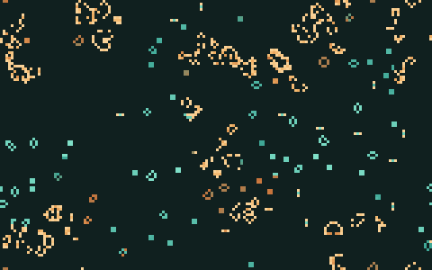
docs/scenes/guides/palettes-age.json and palettes-state.json.Pick a palette in the app
- One automaton. In the CAs pane, each automaton’s card has a Palette list with the built-in palettes and any the scene has of its own. A JACA automaton has two, +1 palette and −1 palette, each with a colour button beside it that sets a single colour instead.
- The Palettes window (CA → Palettes…) shows every palette as a swatch on its own background, so the light ones (Candy, Glacier, Desert and Paper) look right. Choose what to colour under Apply to, every automaton or one, then click a swatch to apply it. Hovering over a swatch, or moving between swatches with the arrow keys after a click, previews it on the grid; Enter applies it.
On a field that several automata share, only the first automaton’s palette shows, and the grid’s background and stage colours always come from the first automaton’s palette (see Several automata at once). If a palette change seems to do nothing, change the first automaton’s instead.
Make your own palette
The lower half of the Palettes window edits a palette:
- Start from a palette that is close to what you want, and give it a Name.
- Change the Stops: click a colour to change it, x under it to remove it, and + to add one. The first stop colours the youngest cells or lowest states, and the last the oldest or highest. The bar above the stops shows the ramp as JETCARP will draw it.
- Set the Background (empty cells) and the Stage (outside the tiling, and the letterbox around a wallpaper that does not fill its image).
- Save as “name” adds it to the scene’s own palettes; an edited built-in palette is saved as “name copy”. Apply to every CA (or to the CA) saves it and applies it at once.
A palette you make belongs to the scene: it is saved in the scene file and travels with it, so whoever
opens the scene sees your colours. To use it in another scene, copy its entry from the first scene’s
palettes list (see Scene file format), or apply it again in the app.
You can also write colours directly wherever a palette is named in a scene or a script: #4fc3ff is
one colour, and #103050-#4fc3ff a ramp from the first to the last, with any number of stops between.
The same works for the --palette options of jetcarp wallpaper, jetcarp sheet,
jetcarp hashlife, jetcarp pile and jetcarp media render.
Choose how cells are coloured
Every automaton has a Colour by setting, in the CAs pane, as color_by in a scene, and as the
color_by option of add_ca and update_ca in a script:
| Setting | What it shows |
|---|---|
Auto (auto, the default) | The rule’s natural colouring: age for Life-like, Generations and similar rules; every state for the cyclic and Hodgepodge rules; heights for sandpiles; values for Lenia; fixed colours for WireWorld, the forest fire and von Neumann’s automaton |
Age (age) | How long each cell has been in its state (see below) |
State (state) | One colour per state, spread evenly from the first stop to the last |
Row (row) | Each live cell by its height in the picture, top to bottom across the whole palette: a gradient for elementary rules, or any tiling |
The full table of what Auto means for each family is in the reference.
Age colouring
Each live cell carries an age: the number of generations it has been in its current state, starting at 1 when it is born or changes state. Coloured by age, a newborn cell takes the palette’s first stop, and older cells move along the palette on a logarithmic scale, reaching the last stop at an age of 400. So a still life ends at the last stop, an oscillator flickers near the start, and the debris of a soup shows its own history: the places still active at the young end, the parts that settled long ago at the old end. The figure at the top of this page shows it.
A few things to know:
- Choosing a palette for it. Some palettes end on a bright stop, such as Verdigris, so that settled patterns stay vivid; others, such as Ember, end on a dark stop close to their background, so that settled patterns fade and the active regions stand out instead.
- HashLife resets ages. After a HashLife jump every live cell has age 1, so the colours start over (see HashLife and very long runs).
- Ages are part of the state. They are included in the state hash, so two runs that look the same in state colouring but differ in age have different hashes.
- Media use states. The animations that
jetcarp mediamakes colour cells by state, never by age, so that their loops close seamlessly (see Pictures and animations).
JETCARP makes no claim for age colouring: other programs, such as Chris Rowett’s LifeViewer, colour cells by age and did so first (see What is new in JETCARP).
On the command line and in scripts
jetcarp paletteslists the built-in palettes with their background colours, andjetcarp palettes --jsongives their stops, backgrounds and stages as data.- Commands that draw pictures take
--palette NAMEto colour every automaton with one palette:jetcarp wallpaper,jetcarp sheet,jetcarp hashlife,jetcarp pile(sandpile heights, with--reverseto run the palette the other way),jetcarp library renderandjetcarp media render(in place of the media’s own house style). - In a script,
w.add_ca(rule, #{ palette: "Tide", color_by: "age" })sets an automaton’s palette and colouring,w.update_ca(id, #{ palette: "Ink" })changes it, andw.save_png(path, #{ palette: "Paper" })draws one picture in another palette without changing the world.jetcarp("reference.palettes")returns the built-in palettes as data. - In a scene, each automaton’s
palette(and, for JACA,palette_neg) andcolor_byfields, and the scene’s ownpaletteslist (see Scene file format). - Screensaver profiles and rotations can replace every automaton’s palette and colouring with their own, without changing the scene.
Reseeding
Most worlds settle down sooner or later: a Life soup turns to ash, Brian’s Brain dies out, a sandpile stops. Reseeding puts new life into a world: once, by hand, or automatically, through policies that fire when the world has settled or every so many generations. It is what keeps a wallpaper or a screensaver lively for hours. Reseeding works the same way in the app, on the command line, in scripts, through MCP and in scene files, and every reseed is planned from the world’s own random state, so a reseeded run replays exactly.
The three modes
| Mode | What it does | Settings (defaults) |
|---|---|---|
random | Every cell flips with a probability: dead cells come alive, live or dying cells die | flip (0.05) |
rain | Drops fall on random cells: small, roughly round patches in which each dead cell comes alive with a probability. Rain only adds cells | drops (24), min_size and max_size in tiles across (2 and 10; small drops are more likely), density (0.5) |
blobs | A few large patches with a wobbly outline; every cell inside is set alive or dead at a set ratio, overwriting what was there | count (1), min_radius and max_radius as fractions of the grid’s shorter side (0.06 and 0.18), live (0.35) |
Sizes are measured in typical tiles, so a drop six tiles across looks the same on squares, hexagons, mixed tilings and aperiodic patches; on wrapped grids, drops and blobs wrap across the edges. A reseed writes into the field of every running automaton (sandpiles excepted), or into one automaton’s field if you name it. New live cells are in state 1, with age 1.
On a JACA field, whose live cells are +1 or −1, each mode also takes a sign:
either (the default: each drop or blob is all +1 or all −1, at random; in random mode, each cell),
mixed (each new cell +1 or −1 at random), alternate (drops and blobs alternate, and the first sign
changes with every reseed), pos or neg. Other fields ignore it.
Reseed now
- In the app: Seed → Reseed now → Random, Rain or Blobs, or the Reseed now buttons in the Reseed pane. Their settings, and which automaton they aim at, are under Reseed now settings in the same pane (Defaults puts them back).
- On the command line:
jetcarp run scene.json --reseed-now rain --gens 500reseeds once before running. The mode is a name (random,rain,blobs, optionally with a JACA sign:rain:neg) or JSON:--reseed-now '{"kind":"rain","drops":40}'. - In a script:
w.reseed("blobs")reseeds every running automaton’s field, andw.reseed(id, #{ kind: "rain", drops: 30, min_size: 2, max_size: 8 })one automaton’s.
A reseed by hand also restarts the cooldown of every automatic policy.
Automatic policies
A policy has a mode, a trigger (when), a cooldown, and optionally a target automaton (ca; without
one it reseeds every running automaton). There are two triggers:
everyfires everygensgenerations (1 means every generation: a continuous drizzle).settledfires when the world has settled. It is checked every 16 generations once the cooldown is over, and fires when any one of these holds:- fewer than
activityof the cells (default 0.002, that is 0.2%) changed in each of the lastfor_gensgenerations (default 60); - the number of cells changing each generation has repeated with a period of at most
cycle(default 12, at most 64) over those generations, which means only oscillators and gliders are left (Life’s ash keeps about 1% of its cells blinking, so a threshold alone would never see it settle); - an exact repeat of the whole state with a period of at most
periodwas seen (off by default); - the running fields are empty;
latestgenerations have passed since the policy last fired, whatever the activity (off by default). This makes sure a screensaver never stalls.
- fewer than
The cooldown is the number of generations after a policy fires (or is installed, or a reseed by hand) during which it cannot fire, so that a new seed has time to develop; a settled policy starts counting quiet generations only once it is over.
Policies run independently of each other, and that can surprise you: a frequent every policy keeps
the world busy, so a settled policy beside it may never see it settle. Here Life ran for 3,000
generations with blobs when settled and ten drops of rain every 500 generations:
$ jetcarp run crates/jetcarp-core/data/scenes/life.json --gens 3000 \
    --reseed '[{"mode":"blobs","when":"settled","cooldown":200},{"mode":{"kind":"rain","drops":10},"when":{"kind":"every","gens":500}}]'
...
reseed:     blobs when settled: fired 0 times, last at -
reseed:     rain every 500: fired 6 times, last at 3000
Giving the settled policy a latest (Anyway after in the app) makes it fire anyway.
The Reseed pane
Seed → Reseed opens the Reseed pane. At the top is a graph of the share of cells that changed in each of the last 512 generations, on a log scale, with the settled thresholds in orange, automatic reseeds in pink and reseeds by hand in blue; beside it are the current activity, the population and the generation.
Presets install a ready-made set of policies with one click. Their drop counts are tuned for a grid of 200 × 140 squares and scaled to the size of yours:
| Preset | Policies |
|---|---|
| Screensaver | Blobs when the world settles (or after 2,400 generations at the latest, cooldown 150), and a light rain every 400 generations: keeps any rule lively without turning it to noise |
| Gentle drizzle | A few small rain drops every 30 generations |
| Continuous rain | One or two tiny drops every 3 generations |
| Storm | Many large drops every 8 generations |
| Blobs when settled | Two large patches at 35% live when the world settles, or after 4,000 generations at the latest (cooldown 150) |
| Full refresh when settled | Flip 25% of all cells when the world settles (cooldown 300) |
Type a name and press Save as preset to keep the current policies as a preset of your own (saved in the app’s settings and shown with a ★); Delete… removes one.
Automatic policies lists the policies, each with a checkbox that switches it on and off, its mode and settings, the Sign when a JACA field is involved, When (Settled, with Activity below, Repeating up to, Exact period up to and Anyway after; or Every N gens, and Continuous for every 3 generations), the Cooldown, and which automaton it reseeds. Each shows how often it has fired. Add policy and Remove all do what they say. Your edits are applied a moment after you stop changing them, as one logged command, so they are saved with the scene.
Seed → Auto reseed switches all the policies on or off at once; when there are none, it installs a preset: Screensaver, unless you choose another (one of yours too) under Seed → Auto reseed installs in the pane’s presets.
From the command line
jetcarp run --reseed installs policies before the run: one policy as a JSON object, or a list. The
mode and the trigger can be given by name, with their defaults ("rain", "settled"), or as objects
with any of their settings. The report has a line per policy saying how often it fired, and --save
keeps the policies in the saved scene, where jetcarp verify replays them.
In a script
let w = load_scene("life.json");
w.set_reseed([
    #{ mode: "blobs", when: #{ kind: "settled", latest: 2400 }, cooldown: 150 },
    #{ mode: #{ kind: "rain", drops: 3 }, when: #{ kind: "every", gens: 400 } },
]);
w.step(5000);
print(w.reseed_status());   // how often each policy fired, and recent activity
w.set_reseed([]);           // remove them
In a scene
A scene keeps its policies in its command log (a set_reseed command), or, to start with them, in
its top-level reseed list. Written out in full, a policy looks like this:
{
  "mode": {"kind": "rain", "drops": 10, "min_size": 2.0, "max_size": 10.0, "density": 0.5},
  "when": {"kind": "settled", "activity": 0.002, "for_gens": 60, "cycle": 12, "latest": 2400},
  "ca": 2,
  "cooldown": 200,
  "enabled": true
}
Every field but mode and when may be left out. See
Scene file format.
Reseeding and reproducibility
Which cells a reseed touches depends only on the tiling and the world’s random state, not on the cells’ current states, and the policies’ progress is part of the state hash. So a reseeded run gives the same hash at any thread count and on the CPU or the GPU, and settled policies are checked only every 16 generations so that the GPU can run whole batches between checks (see Reproducibility).
Screensavers and rotations
A screensaver profile can carry reseed policies of its own, which replace the scene’s while it shows; their drop counts are scaled to the size of the screen’s grid, as the presets are. A rotation can give its items reseed policies, or none at all.
Wallpapers, screensavers and the background host
JETCARP can keep cellular automata running on your screen in four ways:
- Screensaver mode in the app fills the screen (or several) with a scene until you press Esc. It runs while the app is open.
- The background host is a separate program,
jetcarp host, that keeps scenes running with no app window: in a window of its own, or as the live desktop background behind your windows. It can start at login. - The system’s screen saver. On Windows and macOS, JETCARP can be added to the system’s own list of screen savers. GNOME has no such list; JETCARP’s lock-screen mode does the job there.
- Still wallpapers, pictures cut to fit your monitors, are covered in Pictures and animations.
What any of these shows is a screensaver profile, a rotation (a list of items that change over time), a scene file or a Quick Start entry. For a first, step-by-step setup, see Your first live wallpaper.
What works on which system
| Linux with GNOME | Other Linux desktops | Windows | macOS | |
|---|---|---|---|---|
| Screensaver mode in the app | Yes | Yes | Yes | Yes |
| Background host in a window | Yes | Yes | Yes | Yes |
| Live desktop background | With JETCARP’s GNOME extension (GNOME Shell 50) | No: the host shows a window instead | Yes, under the desktop icons | Yes, behind the desktop icons, on every Space |
| Live lock screen | Yes, through the extension | No | No | No |
| In the system’s screen saver list | No (use the lock screen instead) | No | Yes (JETCARP.scr) | Yes (JETCARP.saver) |
| Menu for the host | In the top bar, from the extension | None | In the notification area | In the menu bar |
| Still picture as the desktop background | Yes | No | Yes | Yes |
| Start the host at login | Yes | Yes (an autostart entry) | Yes | Yes |
None of this needs administrator rights: everything JETCARP sets up lives in your own folders and settings, and Uninstalling undoes it.
What has been tested
These features were tested by hand in November 2026 on three machines, on the code of JETCARP’s predecessor CART just before it took its present name. The renamed program has not yet been tested on these machines again.
- Fedora 44, GNOME 50.6 on Wayland, one monitor: the live desktop background, the top-bar menu, and the lock screen in both modes, including unlocking with a real password and stopping the host by force while locked (GNOME’s own background came back and unlocking still worked). Several monitors have only been tried in a headless GNOME session. Since those tests, the part of the extension that keeps the host’s windows out of the overview and the window switcher has been rewritten, and the new version has not yet been tested in a real GNOME session.
- Windows 11 Home (version 26H2) on a laptop with two graphics adapters, with and without a second monitor: the live desktop background under the icons (including after Explorer restarts and after a change of display scaling), the screen saver (install, preview, starting after the idle time, removal), the still picture, sleep, and the pauses on battery and when busy.
- macOS 27.0.1 on an M2 Max MacBook Pro, with and without an external monitor: the live desktop background, the screen saver (preview, starting after the idle time, two screens, sleep while it runs, removal), sleep with the lid closed, the still picture on one screen, and the pauses on battery and when busy.
Not tested yet: starting at a real login on any of the three (the entries are written and removed correctly, but no one has logged in with them), a fresh boot on Windows, Linux desktops other than GNOME, Intel Macs, and any other versions of these systems.
Screensaver mode in the app
View → Screensaver mode (F12), or Start the screensaver in the Screensaver pane, hides every control and runs the screensaver; Esc leaves it. It runs full screen on the app’s monitor, or on the monitors chosen in the Display pane.
View → Screensaver settings… opens the Screensaver pane:
- Show chooses what it runs: One profile, A rotation, The current world, A scene file or
A Quick Start entry (such as
rule:B3/S23). - While it runs has the caption (Show what is running (the rule and the grid), its corner, size, whether it includes the generation count, and how long it stays up after each new item; press I while the screensaver runs to show or hide it), Keep the computer awake while it runs, Leave on any key or mouse movement (else Esc only), Hide floating and popped-out windows, Start AI control, and Hide the pointer after a delay.
- Background host controls the host (see below).
- Profiles lists and edits the screensaver profiles (see below).
The app can also start straight into screensaver mode, for example from a desktop shortcut:
jetcarp --screensaver --rotation "Wolfram series" --quit-on-exit
jetcarp --screensaver --profile Life --monitors 0,1 --span --cell-px 3 --caption
jetcarp --screensaver --quickstart rule:B3/S23 --keep-awake
--scene FILE shows a scene, --mirror shows the same view on every monitor instead of one canvas
across them (--span, the default), and --quit-on-exit closes the app when the screensaver ends.
jetcarp --help lists every option. A running app with control switched on (Tools → AI control… or
jetcarp --control) can be steered from a terminal with jetcarp app screensaver on --profile NAME,
jetcarp app next, jetcarp app profiles and the other jetcarp app commands.
Screensaver profiles
A profile is a named, complete setup for the screensaver: what to show (a scene kept in the profile, a scene file or a Quick Start entry), and optionally a palette and colouring for every automaton, reseed policies that replace the scene’s own, the cell size in pixels, whether to rebuild the tiling to fill the screen, the speed, the GPU simulation, and how many minutes it gets in a rotation. JETCARP has eleven built in: Life, HighLife, Day & Night, Hexagonal Life, Brian’s Brain, Star Wars, Triangles, Snub square Life, Penrose waves, Cyclic spirals and Hodgepodge.
To make your own, set up a world as you like it and press Save current world as profile, or select a profile and change it in the editor below the list. The easiest way to tune one is to press Try in this window, adjust it with the Reseed pane, the palettes and the Run menu, and then press Update from the current world. Tune for this rule runs small copies of the profile’s world with each of the reseed presets and scores how lively each keeps it. Editing a built-in profile saves your own copy under the same name; Revert to built-in goes back.
Profiles are JSON files, one each, in the screensavers folder of the settings folder (see
Folders). Export… saves one to share, Import… adds files, and Reload
reads them again after editing them by hand.
The background host
The host runs as its own program, so its scenes keep going when the app closes, and only one runs at a time. It shows one or more screens, each running a rotation either in a window or as the desktop background, on a chosen monitor or across all of them.
Start and stop it from the Background host section of the Screensaver pane (Start, Stop, Pause, and ◀ ▶ for the previous and next item), from its menu, or from the command line:
$ jetcarp host start --rotation "Wolfram series"
running, pid 676359, up 0.0s, 90 MB, GPU AMD Radeon 8060S Graphics (RADV STRIX_HALO)
screen 0: Wolfram series · W0 (1 of 256) · generation 4 · 57600 cells
$ jetcarp host next
running, pid 676359, up 3.0s, 90 MB, GPU AMD Radeon 8060S Graphics (RADV STRIX_HALO)
screen 0: Wolfram series · W1 (2 of 256) · generation 198 · 57600 cells
$ jetcarp host stop
stopped
| Command | Effect |
|---|---|
jetcarp host start [--rotation NAME] [--headless] | Start the host; it keeps running after the command ends. --rotation is for this run only; --headless runs it with no window or menu |
jetcarp host stop, status, pause, resume | Quit it, say what it shows, freeze it, carry on |
jetcarp host next, previous [--screen N] | The next or previous item, on every screen or one |
jetcarp host rotation NAME [--screen N] | Choose a screen’s rotation |
jetcarp host fps N | The most frames per second it draws (1 to 240; default 30) |
jetcarp host caption on|off | Show what is running in a corner, with --corner, --size, --generation on|off and --seconds |
jetcarp host battery on|off | Pause while the computer runs on battery (default on) |
jetcarp host busy PERCENT | Pause while the whole processor stays at least this busy, as during a long search (default 80; 0 never). It carries on once the load is 20 points lower |
jetcarp host wallpaper, still, lock, gnome, saver, login | See the sections below |
The settings are saved in host.json in the settings folder. The app and the command line both write
it and tell a running host to read it again, so a setting changed while the host is stopped applies
the next time it starts (saved; the host is not running). Besides pausing on battery and when busy,
the host also pauses by itself while its desktop background is completely hidden behind other windows
and while the screen is locked and dark. jetcarp host status --json shows what it is holding for,
under held.
On Windows and macOS the host has an icon in the notification area or the menu bar, and on GNOME the extension adds one to the top bar. Its menu names what is showing and has Next, Previous, Paused, Show on the desktop, Rotation, Open JETCARP, Start at login and Quit (on GNOME, also Start JETCARP host while it is stopped).
The live desktop background
Tick Show on the desktop in the Background host section, or run jetcarp host wallpaper on. To
put different rotations on different monitors, set up one screen per monitor:
jetcarp host wallpaper on --screen 0 --monitor 0
jetcarp host wallpaper on --screen 1 --monitor 1 --rotation "Classics, hourly"
jetcarp host status lists the monitors by number. A screen given no monitor fills every monitor no
other screen claims, and jetcarp host wallpaper off turns the screens back into windows.
GNOME needs JETCARP’s GNOME Shell extension, JETCARP live desktop, which shows the host’s windows as the background of the desktop, the overview and the lock screen, and adds the top-bar menu. It supports GNOME Shell 50.
jetcarp host gnome install    # copy it into place and switch it on; log out and back in once
jetcarp host gnome status     # "The GNOME extension is running."
jetcarp host gnome remove
The Background host section shows the same status, with an Install button. Without the extension the host shows a plain window and says why, so nothing is left covering the desktop. The extension only places copies of the host’s picture in GNOME’s background; it takes no part in unlocking, and if the host stops, GNOME’s own background comes back.
On the lock screen (jetcarp host lock, or On the lock screen in the app) the choices are off
(GNOME’s own background), live (the default: the scene, blurred behind the clock, with GNOME fading
the screen to black as usual) and screensaver (the scene stays sharp and lit until someone reaches
for the password box). In screensaver mode the screen and the computer stay awake while locked;
--awake MINUTES (default 30, 0 for never) lets the screen go dark after that long.
Windows: the host puts a window of its own under the desktop icons, one per monitor, with no extension needed. macOS: one borderless window per monitor at the desktop’s level, behind the icons, on every Space and ignoring the mouse; the host has no Dock icon while it shows only wallpaper. Other Linux desktops are not supported yet: the host shows a window instead.
A still picture. With jetcarp host still on (Leave a still picture when it stops), the host
sets a picture of its scene as the desktop’s own background when it stops, and while the live one
cannot be shown, through the system’s own setting. Your own picture is remembered and put back when
the still or the live background is turned off, unless you have chosen another picture in the
meantime. It is off by default.
The system’s screen saver
jetcarp host saver install adds JETCARP to the system’s list of screen savers and opens the system’s
screen saver settings, with JETCARP to choose. --rotation NAME chooses what it runs (otherwise the
first screen’s rotation); in the app, the same choice is Screen saver runs, with an Install button.
jetcarp host saver status says whether it is installed, and remove takes it out.
- Windows. A copy of JETCARP’s windowless launcher is made at
%LOCALAPPDATA%\JETCARP\JETCARP.scrand selected in Screen Saver Settings, as right-clicking a.scrfile and choosing Install would. It reads JETCARP’s settings each time it starts, so changes apply at once, and its Settings button opens the JETCARP app. It needsjetcarpw.exe, the windowless launcher, besidejetcarp.exe; a build from source makes it withcargo build --release -p jetcarp --features windows-launcher. Removing it also clears the selection if JETCARP was the chosen screen saver. - macOS. macOS runs screen savers in a sandbox that cannot read JETCARP’s settings, so installing
builds
~/Library/Screen Savers/JETCARP.saverwith the rotation and every item’s scene copied inside it, signs it for this machine, and opens System Settings where screen savers are chosen (System Settings, Wallpaper, Screen Saver… on macOS 27). Install it again after changing the rotation. It needslibjetcarp_saver.dylibbeside thejetcarpprogram; a build from source makes it withcargo build --release -p jetcarp-saver. - GNOME has no list of screen savers. Use the lock screen’s screensaver mode instead:
jetcarp host lock screensaver --awake 30.
Start at login
jetcarp host login on (or Start at login, in the app or the host’s menu) makes the host start when
you log in; jetcarp host login off stops that. It uses each system’s own per-user mechanism:
| System | What is written |
|---|---|
| Linux | ~/.config/autostart/jetcarp-host.desktop |
| macOS | ~/Library/LaunchAgents/com.jimmieprodgers.jetcarp.host.plist (it takes effect at the next login) |
| Windows | The value JETCARP under HKEY_CURRENT_USER\Software\Microsoft\Windows\CurrentVersion\Run |
The entry runs jetcarp host serve (on Windows through jetcarpw.exe when it is there, so no console
window opens) at the path the program has now. If you move the program, turn the setting off and on
again. A host already running is left alone.
More: Rotations, Reseeding, Folders and Uninstalling.
Rotations
A rotation is what the screensaver or the background host shows over time: a list of items, each a screensaver profile, a scene file, a Quick Start entry or a whole series of rules, played in order, shuffled, or one a day. Each item has the conditions that end it, such as a number of minutes, the world settling, or a time of day, and can be limited to certain days and hours. A rotation can also have a short script that decides when to move on. This guide covers the built-in rotations, using one, and making your own.
The built-in rotations
| Rotation | What it shows |
|---|---|
| Wolfram series | All 256 elementary rules, each drawn line by line to the bottom of the screen, then the next (4-pixel cells, in Ink) |
| A classic a day | A different classic each day, restarting if it ends: Life, Langton’s ant, a forest fire, cyclic spirals, the turmite LLRR, Penrose waves and Hodgepodge. The background host runs this one unless told otherwise |
| Classics, hourly | The same classics in a new random order, an hour each |
| Until it settles | Life, HighLife (B36/S23) and B368/S245 with no reseeding, each until it settles (at most 30,000 generations), then the next |
Use a rotation
- Screensaver mode in the app: in the Screensaver pane, set Show to A rotation and choose it
under Rotation, or start the app with
jetcarp --screensaver --rotation "Wolfram series". - The background host: choose it under Rotation in the pane’s Background host section, or run
jetcarp host rotation "Classics, hourly"(add--screen Nfor one screen of several).jetcarp host start --rotation NAMEruns one for that run only. - The system’s screen saver:
jetcarp host saver install --rotation NAME, or Screen saver runs in the app. On macOS the rotation is copied into the screen saver, so install it again after changing the rotation (see Wallpapers).
While a rotation runs, the ◀ and ▶ buttons in the pane, Next and Previous in the host’s menu,
jetcarp host next and previous, and jetcarp app next for the app’s screensaver skip between items.
A rotation that names an item that no longer exists (a deleted profile, say) leaves it out; one that
cannot be found at all shows Life instead.
Make a rotation in the app
In the Screensaver pane, set Show to A rotation. Under the rotation’s name are Edit, New, Duplicate and, for one of your own, Delete (for an edited built-in rotation, Revert to built-in). The editor has:
- Name, and Order: In order, Shuffled (a new random order each time through) or One a day (one item per calendar day, the next one tomorrow; it restarts if it ends during the day). Default sets the minutes for items with no ending of their own; untick it and such items run until something else moves on.
- Settings for every item: a cell size, a speed, a palette, whether periodic tilings are rebuilt to fill the screen, and No reseeding. These apply to every item that is not a stored profile.
- The items. Add profile, Add scene…, Add series (one item per rule, for example every
Wolfram rule) or a Quick Start entry’s handle typed into the box (such as
rule:B3/S23,langtons-ant, an atlas entry’satlas:…or one of your ownfind:…; press Enter). Each item can be moved and removed, and has:- Ends (any of these), from Add ending: After minutes, After generations, When settled (the same test the reseed policies use, with an optional limit in generations), On low activity (under a share of cells changing, for a number of generations), When finished (a rows rule reaches the bottom, or nothing can change any more), and At a time of day. With no ending, an item takes its profile’s minutes, else the rotation’s default.
- Hold: seconds to keep showing the finished world before moving on.
- Only at certain times: the days of the week, and hours Between two times (which may cross midnight). Outside them the item is skipped.
- Settings for this item, as above, for this item alone.
- For a series: the Rules (a series name such as
WorHexW, a template with{n}, or a list), the Tiling, From and To, and the Seed.
- Script: Add a script (see below).
Save keeps it, Save and start runs the screensaver on it at once, and Close discards the edits. Editing a built-in rotation saves your own copy under the same name.
Rotation files
Each rotation of your own is a JSON file in the rotations folder of the settings folder (see
Folders), so rotations can be written by hand, kept and shared. The app,
the host and the Windows screen saver read the same files; the macOS screen saver gets a copy when it
is installed. This one shows Brian’s Brain until it settles,
then Langton’s ant for ten minutes, and from 10 pm to 6 am also the 256 elementary rules:
{
  "name": "Evenings",
  "description": "Brian's Brain until it settles, then a Langton's ant for ten minutes; the Wolfram rules at night.",
  "order": "in_order",
  "default_minutes": 5.0,
  "items": [
    {"source": {"kind": "profile", "name": "Brian's Brain"},
     "end": [{"kind": "settled", "latest": 20000}], "hold_s": 3.0},
    {"source": {"kind": "quick_start", "id": "langtons-ant"},
     "end": [{"kind": "minutes", "minutes": 10.0}],
     "look": {"cell_px": 4.0, "speed": 240.0}},
    {"source": {"kind": "series", "rules": "W", "from": 0, "to": 255},
     "end": [{"kind": "done"}], "hold_s": 3.0,
     "schedule": {"from": "22:00", "to": "06:00"},
     "look": {"cell_px": 4.0, "palette": "Ink"}}
  ],
  "script": "if s.population == 0 { \"next\" }"
}
| Field | Meaning |
|---|---|
name, description | Shown in the app and the host’s menu |
order | in_order (default), shuffle or daily |
default_minutes | Minutes for items with no ending of their own (5 if left out); null lets them run until something else moves on |
look | Settings for every item that is not a stored profile: cell_px, speed (generations per second), refill, gpu, palette, color_by, and reseed (a list of reseed policies; [] for none). The app’s editor sets all but gpu and color_by, and of reseed only No reseeding |
items | The items, in order |
script | Rhai code run about once a second (see below) |
An item has a source, which is one of {"kind": "profile", "name": …}, {"kind": "scene", "path": …},
{"kind": "quick_start", "id": …} and {"kind": "series", "rules": …, "from": …, "to": …, "family": …, "boundary": …, "seed": …} (a series becomes one item per rule, on a 200 × 140 grid of the
family, square and dead edges by default). It may also have a label, a list of end conditions, a
hold_s in seconds, its own look, and a schedule with days (mon to sun) and from and to
times. The end conditions are {"kind": "minutes", "minutes": …}, {"kind": "generations", "gens": …},
{"kind": "settled", "latest": …} (latest optional), {"kind": "low_activity", "below": …, "for_gens": …}, {"kind": "done"} and {"kind": "clock", "at": "07:30"}.
A rotation’s script
A rotation’s script runs about once a second while the rotation plays. It sees a map s describing
what is showing now, and a map state in which it can keep anything it likes between runs:
In s | Meaning |
|---|---|
index, count, label, n | The item’s number (from 0), how many items there are, its label, and its rule number in a series (else ()) |
generation, seconds | Generations and seconds since the item started |
population, cells, activity | Live cells, all cells, and the share of cells that changed last generation (or () when it was not measured) |
done, settled | Whether nothing can change any more, and whether the world has settled |
hour, minute, weekday | The local time; weekday 0 is Monday |
Its answer decides what happens: nothing (or "continue") carries on, "next" and "previous" move
on, "reseed" reseeds the world now, a number goes to that item, and #{ item: "label" } goes to the
item with that label. The script runs with tight limits on how much work and memory it may use, and
its print output is discarded. New scripts start from this one:
// Runs about once a second. `s` describes what is showing, `state` keeps
// anything you like between runs. Answer "next", "previous", "reseed",
// an item number, or #{item: "label"}. Anything else just continues.
if s.generation > 20000 { "next" }
This is a different, much smaller language environment from jetcarp script:
none of the scripting API’s functions are available in it.
More: Wallpapers, screensavers and the background host and Reseeding.
Searching for patterns
This page is being written.
The pattern library
This page is being written.
Packs: importing, exporting, checking
A pack is how JETCARP shares data: patterns, ant and turmite runs, Quick Start entries, search runs, pictures and ratings, in files that any program can read. Every file is named or listed by its SHA-256 hash, and every version is signed by its publisher, so whoever receives a pack can check that nothing was changed on the way and who made it. JETCARP also checks every pattern’s id against the pattern itself, and runs a sample of the patterns again before trusting them.
This guide covers checking and importing a pack you were given, then publishing and exporting your own. The files themselves are described in Pack format.
Stores and exports
A pack comes in one of two layouts, and every command here takes either:
- A store is a folder that keeps every version of one or more feeds. A feed is a named series
of versions, such as
penrose-finds. Files in a store are named by their hashes (objects/sha256/…), so a new version adds only the files that changed, and the store can be copied to any static web host as it is. - An export is one version laid out with readable names for a single download: a
README.md, aCITATION.cff, aLICENSE, the manifestpack.json, and the tables as Parquet files undertables/.
To send someone a pack, send the export folder, for example as a zip. JETCARP 0.4 imports from a folder, so unpack a zip or tar first.
Check a pack
jetcarp pack check reads a pack and checks all of it, without importing anything. It checks the
format, the publisher’s signature, the hash and size of every file, and every id:
$ jetcarp pack check penrose-finds-2026.11
sha256:a968036b…: feed penrose-finds, by SHA256:yNFIDrcM3AiT87AjIHMwLfCRBHMOW4KZm5X6pwQx1A8 (Ada Example), checking every object
…
checked sha256:a968036b… (feed penrose-finds, SHA256:yNFIDrcM… Ada Example, signed by its publisher)
  9 objects checked (213869 bytes)
The first part is the version id: the hash of the manifest, which in turn lists the hash of every
file. Two packs with the same version id are the same pack. The SHA256:… value is the publisher’s
key fingerprint, the same form ssh-keygen -l prints. A name after it is one the publisher gave
themselves, and nothing more: trust a publisher by their key, for instance one they list on their
website.
If any file was changed, the check fails and says which:
Error: part sha256:d7762c49… is altered or truncated
A pack that its publisher didn’t sign is refused unless you add --allow-unsigned. A store with
several feeds needs --feed NAME, and --manifest sha256:… picks a version other than the newest.
Import a pack
jetcarp pack import runs the same checks and then merges the pack into your library:
$ jetcarp pack import penrose-finds-2026.11
…
imported sha256:a968036b… (feed penrose-finds, SHA256:yNFIDrcM… Ada Example, signed by its publisher)
  9 objects checked (213869 bytes)
  patterns: 3 added, 0 merged, 0 flagged needs_reverify
  sightings 3, ratings 0, ants 0, Quick Start 0, media 0, searches 0, retracted 0
  verified again (sample): 3 of 3 passed, 0 skipped, 0 failed
What happens to each kind of record:
- Patterns are merged by id. A pattern you don’t have is added with its finder, the date it was found, and the publisher’s name, tags and notes for it. A pattern you already have keeps your own name, tags, notes, rating and state: importing never overwrites your curation, so a later version that renames a pattern changes nothing for one you already had. Sightings are counted per search, so importing the same pack twice changes nothing.
- Patterns from another engine version. A pattern whose tiling geometry or rule meaning differs
from this version of JETCARP’s is kept and flagged
needs_reverify.jetcarp library reverifychecks it again. - Sample verification. After merging, JETCARP runs 3,000 of the new patterns again (fewer if the
pack has fewer), chosen at random but seeded by the version id, so the same pack always checks the
same sample.
--verify fullruns every new pattern,--verify noneskips this step,--sample Nchanges the sample size, and--verify-seconds Scaps the time (600 by default). - Search runs become a paused explore job, so
jetcarp jobs status,jobs runsand the atlas work on them as on a search you ran yourself, andjetcarp jobs resumecontinues it. - Quick Start entries appear in the Quick Start menu.
- Ratings are kept under each rater’s name, as the pack gives it.
- Retractions. A publisher can withdraw a record in a later version. Importing that version flags the record as retracted, with the reason, and never deletes your copy.
--strict refuses a pack that has two different rows for one record id, instead of keeping the
first. --library FILE imports into another library file than your usual one.
JETCARP never runs code from a pack. A pack holds data. A scene’s script is a list of steps,
naming which automata run and when to move on (Scene file format),
not a program.
Your publisher key
Every pack you make is signed with your publisher key, an Ed25519 key that JETCARP keeps in its
settings folder. jetcarp pack key makes one the first time and shows it after that:
$ jetcarp pack key
made publisher key SHA256:yNFIDrcM3AiT87AjIHMwLfCRBHMOW4KZm5X6pwQx1A8
  ssh-ed25519 AAAAC3NzaC1lZDI1NTE5AAAAIGPv65+hMLaYJAVXB/chf5oAx0smWQlLyOVymcinItHV jetcarp publisher
  file /home/ada/.config/jetcarp/pack/publisher_ed25519
  not named (packs show the key only; --name to be named)
Your packs show only the key until you give a name. --orcid and --github add those too, and
they appear in each pack’s CITATION.cff:
$ jetcarp pack key --name "Ada Example" --orcid 0000-0002-1825-0097
The key is an ordinary OpenSSH key, so OpenSSH can check JETCARP’s signatures too. In an export’s
folder, with the publisher’s public key in a file allowed as ada ssh-ed25519 AAAA…:
$ ssh-keygen -Y verify -f allowed -I ada -n jetcarp-manifest -s sigs/*.sig < pack.json
Good "jetcarp-manifest" signature for ada with ED25519 key SHA256:yNFIDrcM3AiT87AjIHMwLfCRBHMOW4KZm5X6pwQx1A8
Back up the key file. A new key is a new publisher: later versions of your feeds would be
signed by a stranger. --key FILE signs with an OpenSSH Ed25519 key of your own instead.
Publish your library
jetcarp pack publish writes your library, or part of it, as a new version of a feed in a store.
The store folder is made if it doesn’t exist:
$ jetcarp pack publish --to my-store --feed penrose-finds --title "Penrose finds" --version-label 2026.11
publishing feed penrose-finds (version 1) into /home/ada/packs/my-store
3 patterns read, 3 new rows
…
published penrose-finds version 1 into /home/ada/packs/my-store
  manifest sha256:a968036b954f740867edcd9387c4d87c2ef39424903975cbea85f570154db964
  publisher SHA256:yNFIDrcM3AiT87AjIHMwLfCRBHMOW4KZm5X6pwQx1A8
  patterns       3 rows added, 2 parts
  …
  49117 bytes in all
Run it again later and it writes version 2 of the same feed, storing only what changed. The
feed’s file in refs/ names its newest version and is signed too.
Choose what goes in:
| Option | Effect |
|---|---|
--id ID | Only these records: ids, id prefixes or names (repeat it) |
--query JSON | Only the patterns a library query finds, such as '{"class":"spaceship"}' |
--search UUID | Only these explore searches (repeat it) |
--no-searches, --no-ants, --no-quickstart, --no-media, --no-ratings | Leave that kind out |
Describe it: --title, --description and --version-label (free text such as 2026.11)
go into the manifest and the export’s README. --licence takes an SPDX id; the default is
CC0-1.0, which puts the data in the public
domain. --created fixes the version’s time (RFC 3339, UTC): with the same library, key and time,
publishing gives the same version id, byte for byte.
Withdraw a record: --retract pattern:ID=reason lists it as retracted in this version and every
later one. Earlier versions stay as they were, since every file in them is fixed by its hash, but
anyone importing the new version sees the retraction and its reason:
$ jetcarp pack publish --to my-store --feed penrose-finds --version-label 2026.12 \
    --retract 'pattern:3dec1a434a261b937448693adbeab960=duplicate of a known still life'
Combine versions: --merge FOLDER (or FOLDER@sha256:… for one version) brings another
store’s records into this version. Each keeps its original publisher.
Export a version
jetcarp pack export lays one version out for a single download:
$ jetcarp pack export --from my-store --to penrose-finds-2026.11
exported sha256:a968036b… into /home/ada/packs/penrose-finds-2026.11: 24 files, 222559 bytes
Without --from, it publishes your library first, taking the same options as pack publish, and
exports the result. It keeps the store it made next to the export, in a hidden folder named after
it, for example .penrose-finds-2026.11.store. Use --views to add a views.sql for
DuckDB (see below).
The export’s folder:
| Path | What it holds |
|---|---|
README.md, CITATION.cff, LICENSE | For people and for citation managers, written from the manifest |
pack.json | The manifest; its SHA-256 is the version id |
tables/<table>/…/part-NNNNNN.parquet | The tables, split into parts by class and tiling group |
index/ | The hash of every part |
sigs/, keys/ | The publisher’s signature and public key |
tilings/reference/ | Reference patches for aperiodic tilings, so their pins can be checked |
Ratings and consent
Ratings are about people’s taste, so a pack includes only the ratings of raters who have agreed to
a permanent public release. Record that agreement with jetcarp pack rater, using the name the
library’s ratings give:
$ jetcarp pack rater "Ada Example" --show-name
Ada Example                              rater-17935ea8ceb8a90a  consented 2026-11-12T02:14:37Z, named
- Without
--show-name, a pack lists the rater only by a pseudonymous id such asrater-17935ea8ceb8a90a. --noteslets their notes go in too.--orcidadds an ORCID for a named rater.--withdrawtakes the consent back: later packs leave that rater’s ratings out. Versions already published can’t be changed.- A group rating, made by several people together, goes in only when every member has consented.
Your own curation (the names, tags, notes, star ratings and states you give patterns) is different: it goes into your packs as your annotations, signed with your key.
Read a pack without JETCARP
An export is plain Parquet and JSON, so any data tool can read it. With DuckDB, in the export’s folder:
$ duckdb -init views.sql
D SELECT id, class, period, cells FROM patterns ORDER BY cells;
Polars and pandas read the same files, with read_parquet on a table’s folder.
JETCARP’s source repository also holds an independent reader in Python (tools/jetcarp_pack),
written from the format description alone. It checks hashes, signatures and ids, at the
conformance levels the format defines.
Share a pack
A store or an export is a folder of ordinary files, so any way of moving files works: a zip by email, a static web host, a Git repository with Git LFS, or a data repository such as Zenodo or Hugging Face. To publish a feed for others to follow, copy the whole store to a web host and give people the address. Copy it again after each new version: files already there never change, so only the new ones need uploading.
JETCARP 0.4 doesn’t download packs itself: download the folder first, then import it. Fetching feeds from an address and following them for new versions are planned for a later version.
Pictures and animations
JETCARP draws every picture with its own renderer, straight from a world, so a picture shows the tiles in their true shapes at any size. This guide covers still pictures of a world, desktop wallpapers cut to fit your monitors, animations, and contact sheets that put many runs side by side. Most still pictures carry their scene inside the PNG, so a picture can always be traced back to the run that made it (see Scenes).
| To make | In the app | On the command line | In a script |
|---|---|---|---|
| A picture of the world | File → Export PNG… | jetcarp run --png | w.save_png(path) |
| Desktop wallpapers | File → Export wallpaper… | jetcarp wallpaper | jetcarp("wallpaper.export", #{…}) |
| An animation | jetcarp media render | w.media(#{…}), media(#{…}) | |
| A contact sheet | File → Export contact sheet… | jetcarp sheet, jetcarp quickstart --sheet, jetcarp isohedral --png | sweep(#{…}) writes one picture per run |
A picture of the world
In the app, File → Export PNG… (Ctrl+E) saves the whole tiling as a PNG; the menu shows the size it will be, such as Export PNG (2400 × 1600)…. Export size, just below it, sets the scale: fit gives 2400 pixels on the longer side, and a number gives that many pixels per tile (up to 64). Large images are written in strips, so they need little memory. Tile outlines are drawn where tiles are at least 7 pixels across.
On the command line, jetcarp run writes a picture of the state it ends in:
jetcarp run scene.json --gens 500 --png out.png                # 1600 pixels on the longer side
jetcarp run scene.json --gens 500 --png big.png --max-side 8000
jetcarp run scene.json --gens 500 --png exact.png --scale 6    # 6 pixels per world unit
A tile edge is about one world unit, so --scale 6 gives tiles about six pixels across. Very large
pictures (a small scale on a huge grid) are streamed in strips too.
In a script, w.save_png(path) draws the world at the screen size given by --screen (1920 × 1080
by default), fitted and centred. Its options set the size ([w, h]), scale, max_side,
outlines, a palette for this picture only, and the compression (fast, balanced or high);
it returns the path, the size and the number of bytes.
Desktop wallpapers
A wallpaper is a picture at exactly the size of a monitor, or of several monitors side by side.
In the app, File → Export wallpaper… opens a window that writes desktop-sized PNGs of the world while the app keeps running:
- Size: one of your monitors (as detected), All monitors as a span, a preset, or Custom size.
For a span, Layout gives each monitor as
WIDTHxHEIGHT+X+Y(the wayxrandrprints it; Detected fills in yours), and Write chooses One span image, One per monitor (cut so that they line up across the gaps) or Both. - Fit: Cover (the grid fills the image and is cropped, so no stage colour shows), Contain (the whole grid, letterboxed in the palette’s stage colour), Current view (what the grid view shows now, scaled to the image) or Repeat (a grid with wrapped edges, tiled seamlessly over the image at a chosen tile size).
- Grid: Fresh grid sized for the image builds a new grid of the same tiling, with this world’s automata and seeds, big enough to fill the image at a given number of pixels per tile, and runs it for a given number of generations first (on the GPU if you like). The live world is left alone; Open the fresh grid afterwards replaces it with the new grid if you want to keep it.
- Outlines (Tile outlines when tiles are at least so many pixels across), Palette (as the
automata are, or one palette for all), and the Folder (Choose…; by default the
wallpapersfolder of the output folder). Then Export, and Open folder to see the result.
On the command line, jetcarp wallpaper takes a scene file or a Quick Start id:
$ jetcarp wallpaper life --size HD --gens 200 -o life.png
life.png (1920 x 1080)
$ jetcarp wallpaper life --monitors 2560x1440+0+0,1920x1080+2560+180 --split --gens 100 --palette Glacier
/home/ada/Pictures/JETCARP/wallpapers/Life-on-the-square-grid-1-2560x1440-2026-11-10_18-28-08.png (2560 x 1440)
/home/ada/Pictures/JETCARP/wallpapers/Life-on-the-square-grid-2-1920x1080-2026-11-10_18-28-08.png (1920 x 1080)
| Option | Effect |
|---|---|
--size | WIDTHxHEIGHT or a preset: HD (1920 × 1080), WUXGA (1920 × 1200), QHD (2560 × 1440), WQXGA (2560 × 1600), UWQHD (3440 × 1440), 4K (3840 × 2160, the default), 5K (5120 × 2880), 8K (7680 × 4320), Phone (1080 × 2400) |
--monitors, --split | A span of monitors as WIDTHxHEIGHT+X+Y,…; with --split, one image per monitor instead of the whole span |
--fit | cover (default), contain or repeat (a wrapped grid tiled at --cell-px) |
--center X,Y --scale S | Look at this point of the world at this scale instead of fitting |
--fresh, --cell-px | Build a fresh grid of the scene’s tiling sized to fill the image at --cell-px pixels per tile (default 4), with the scene’s automata and seeds but not its later edits |
--gens, --gpu | Generations to run first, on the GPU where the rules allow it |
--palette, --outline | One palette for every automaton (a name); tile outlines when tiles are at least this many pixels across |
-o, --out | A file or a folder (default: the wallpapers folder of the output folder) |
jetcarp --json quickstart lists the built-in Quick Start entries with their ids (such as life or
langtons-ant); entries of your own are find:… and the atlas’s atlas:…. To show a wallpaper that
moves, see Wallpapers, screensavers and the background host.
Animations
jetcarp media render makes a set of media: a PNG frame for every step, an animation, a poster frame
and a thumbnail.
$ jetcarp media render --scene docs/scenes/automata/turmite-llrr.json --gens 120 --every 2 --no-frames --out llrr
webp   llrr/anim.webp
poster llrr/poster.png
thumb  llrr/thumb.png
- What to render.
--scene FILErenders any scene from its first generation; without--out, the files go tomedia/<file name>in the output folder.--quickstart IDwith a built-in Quick Start entry’s id or number (asjetcarp quickstartlists them) renders that entry’s scene the same way, intomedia/<id>without--out. The other targets come from the pattern library:--pattern ID(a catalogued pattern, shown alone),--quickstart HANDLE(one of the library’s own Quick Start entries:find:IDunder My finds,atlas:…, or a pack’sqs-…),--ant ID(an ant run) and--missing(everything in the library whose media are missing or out of date, limited with--class,--only-patterns,--only-quickstartand--limit). Their media are kept in the library’smediafolder, each file once under the SHA-256 of its bytes (see Library format), and rendered again only when something has changed (--forcerenders anyway).jetcarp media list KIND IDlists a record’s files with their paths,jetcarp media export KIND ID --to DIRcopies them into a folder asframes/0000.png…,anim.gif,poster.pngandthumb.png, andjetcarp media gcdeletes the files no record uses any more (--dry-runlists them first). - How. A pattern alone is shown on an empty field for
--periodsfull periods (default 1), so the animation loops seamlessly; a spaceship’s window moves with it. From the seed, the whole grid runs for--gensgenerations (default 200; row rules one frame per row), with a frame every--everygenerations.--modeoverrides the choice. - Format. With
--format auto(the default), the animation is a GIF when each frame is at most 320 × 320 pixels, the whole animation at most 8 million pixels and 256 colours, and an animated lossless WebP otherwise;--format gifand--format webpchoose one.--no-framesskips the per-step PNGs. - Look. Media have a house style: a fixed set of colours for each kind of field, cells coloured by
state and never by age (so loops close), outlines where tiles are at least 8 pixels across, whole
pixels per cell, about 320 pixels across for a pattern alone and 512 from the seed, and no text.
--palette NAMEuses a palette instead. Media files do not carry the scene inside them.
In a script, w.media(#{ gens: 200, every: 2 }) renders a world from its current state into a new
media folder, and media(#{ pattern: id }) renders library media, with the same options as the
command. The animations in this book are made from their scenes by a separate tool,
docs/tools/render-animations.sh, which uses Python to crop and label the frames.
Contact sheets
A contact sheet lays many small pictures out in a grid, each labelled, to compare rules at a glance.
- Elementary and hexagonal row rules. File → Export contact sheet… draws the world’s first row
rule and the rules after it (64 of them, or all 16 binary hexagon rules) in its palette, and
Contact sheet… on an automaton’s card in the CAs pane does the same for that automaton’s rule.
From the command line,
jetcarp sheet --kind w --from 0 --count 64 --png sheet.pngdoes the same for any range, with--cols,--thumb(pixels per thumbnail),--width(cells across each),--random-row DENSITY(start from a random top row instead of one cell) and--palette. The kinds arew(rules 0 to 255),hexw(0 to 15),hexw3(0 to 19,682),hext(0 to 255),hext3andhext3sum(see Hexagonal row rules). - Sweep folders.
jetcarp sheet --folder FOLDER --runs "#12,#40,n=588" --png picks.pnglays out chosen runs of a sweep, each under its label (--labels) and rule. - Quick Start.
jetcarp quickstart --sheet sheet.pngdraws every built-in entry, numbered asjetcarp quickstartlists them, after--gensgenerations (default 300);--filter TEXTkeeps the entries whose name, rule, family or tiling contains the text. - Isohedral types.
jetcarp isohedral --png sheet.pngdraws all 81 types (see Drawing and editing tiles).
The exploratory search makes contact sheets of its own for reviewing what it found (see Search methods).
Other pictures
jetcarp hashlife … --pngdraws a pattern far in the future: with JETCARP’s renderer up to--max-cellscells (16 million by default), and as a density map beyond that (see HashLife and very long runs).jetcarp objects scene.json --png objects.pngcolours each object of a world by its class: still life, oscillator, spaceship or other.jetcarp library render ID --pngdraws a catalogued pattern’s phases side by side (see The pattern library).jetcarp piledraws a large sandpile (see Large sandpiles).
The still figures in this book are made with jetcarp run --png and the contact-sheet commands, from
the scene named under each, by docs/tools/render-figures.sh.
Large sandpiles
jetcarp pile drops N grains of sand on one tile of an unbounded grid and lets them settle, for N
from one to 2⁶⁴ − 1, on any tiling: the regular grids, every periodic tiling in the catalogue, and
exact patches of the aperiodic ones. It draws the settled pile as a picture, records how it grew, and
saves its progress so a pile that takes hours can be stopped and carried on. The method (it never
builds a tower of N grains, but doubles a smaller pile again and again) is explained under
Very large piles in the sandpile chapter.
Build a pile
$ jetcarp pile --grains 1e6
pile job 1 in /home/ada/.local/share/jetcarp/library.sqlite
pile 1: 1000000 grains on square, step 16/20 (62500 grains), 4.633e7 topplings, 2.8 s; step 17 running 3.0 s
pile 1: 1000000 grains on square, step 18/20 (250000 grains), 7.321e8 topplings, 7.0 s; step 19 running 4.0 s
pile 1: 1000000 grains on square, step 19/20 (500000 grains), 2.909e9 topplings, 15.7 s; step 20 running 1.0 s
done: 1000000 grains, 11583796400 topplings, 296811 sweeps, 20.6 s of toppling
image:   /home/ada/Pictures/JETCARP/piles/2026-11-11_21-20-08_square-1000000/pile.png
preview: /home/ada/Pictures/JETCARP/piles/2026-11-11_21-20-08_square-1000000/preview.png
folder:  /home/ada/Pictures/JETCARP/piles/2026-11-11_21-20-08_square-1000000
job:     1
A million grains take 20 steps, one for each binary digit of 1,000,000, and each step is about four
times the work of the one before. N can be written 1000000, 1e7 or 2^30.
On the GPU, --gpu topples periodic tilings on the graphics card. It gives the same pile, and on
the desktop these numbers come from (a Radeon 8060S), a million grains on squares took 1.7 seconds
instead of 20.6 on 32 CPU threads. Aperiodic tilings are toppled on the CPU.
| Option | Effect |
|---|---|
--grains N | How many grains (default 100,000) |
--tiling ID | Any tiling id: square (the default), hex, triangle, snubsq, cairo, k3-012, ih41, spectre, hat… (see Tiling catalogue) |
--nb edge / --nb touch | Neighbours that share an edge (the default; von Neumann on squares), or that touch at all (Moore on squares) |
--centre cell / vertex / edge | Drop the grains on one tile (the default), or share them among the tiles that meet at a vertex or an edge |
--level N | Aperiodic tilings: the patch level (by default the smallest that should hold the pile, up to 8) |
--gpu | Topple on the GPU (periodic tilings) |
--threads N | CPU threads (default all); the result doesn’t depend on it |
The pile is the same however it is built: on the CPU or the GPU, with any number of threads, in one run or resumed many times.
The pile’s folder
Each pile gets a folder under <Pictures>/JETCARP/piles/, named after when it started, its tiling
and its grains (--out DIR puts it elsewhere):
| File | What it holds |
|---|---|
pile.png | The settled pile, cropped to it, at --px pixels per cell (default 2) with a --margin of empty cells (default 4) |
preview.png | The same picture scaled to --preview pixels on its longest side (default 1024; 0 for none) |
pile.json | What was built and how: tiling, grains, neighbours, centre, the board’s size, the pile’s width and height, the picture’s settings, and a record for every step |
growth.csv | One row per step: grains so far, topplings, sweeps, seconds, the pile’s width and height, the board’s cells, and what toppled it |
look.json | The palette and its direction |
steps/step-NN.pile | The pile after each step, for resuming |
The step files are small, because a settled pile holds at most a few grains per tile: the folder of
the million-grain pile above is 592 KB in all. --no-png skips the full-size picture of a pile too
big to want one.
Colours
Heights run along a palette: height 1 at its first stop and the tallest at its last, with empty
tiles in its background colour. The default is Ember. --palette NAME picks another (jetcarp palettes lists them, or give hex colours), and --reverse runs it the other way. See
Palettes and colouring.
To recolour a pile after it is built, open it in the app’s sandpile window (below), choose the colours, and use Write pile.png, preview.png, and pile.json in these colours.
Stop and carry on
Every pile is a job in your library, like a search, so the usual job commands work on it:
$ jetcarp pile --grains 1e9 --gpu --minutes 0.25 --label big
…
pile 5: 1000000000 grains on square, step 22/30 (3906250 grains), 1.750e11 topplings, 13.5 s
pile 5 paused (at its budget); `jetcarp jobs resume 5` resumes it exactly

$ jetcarp jobs list
    5  pile     paused   2026-11-12T02:21:08Z  pile 5: 1000000000 grains on square, step 22/30 (3906250 grains), 1.750e11 topplings, 13.5 s
    …
--minutes Mor--until UNIX-TIMEstops it after a while, andjetcarp jobs stop JOBor Stop in the app stops it at once.jetcarp jobs resume JOBcarries it on. So doesjetcarp pile --resume JOB-OR-FOLDER, which keeps the pile’s settings and ignores the other options. Add--gputo resume on the GPU again: it is chosen for each run, not stored with the pile.--detachruns the pile in a process of its own and returns at once, sojetcarp jobs status JOBcan follow it.
A pile resumes from its last finished step. A step stopped part way is run again from the start,
and steps get long: the last few steps of a billion-grain pile each take minutes. So give a run
long enough to finish its step. Once two steps have run, jetcarp jobs status and the app show an
estimate of the time left.
In the app
Tools → Large sandpile… builds the same piles. It has the options above, draws the pile as it grows, and shows each step’s progress and the time left. Stop (resumable) stops the pile, and Resume carries it on from its last finished step; a pile stopped elsewhere (from the command line, or the Hunts… window) can be resumed there too.
From scripts and other tools
The same piles are jetcarp search pile (the pile as a search strategy, taking the same options),
sandpile_pile(#{ … }) in Rhai scripts (see Scripting),
and the MCP server’s search tools (see MCP tools).
HashLife and very long runs
HashLife, Bill Gosper’s algorithm of 1984, jumps a pattern millions or trillions of generations
ahead in a moment. It cuts the plane into blocks, remembers how each block evolves, and treats equal
blocks anywhere in space and time as one, so a pattern that is regular, such as a glider gun and its
stream, costs almost nothing to run far ahead. JETCARP’s HashLife was written for it from the
published algorithm, and it works on every periodic tiling, not just the square grid. This guide
covers what HashLife can run, the two ways of jumping, the HashLife view window, the
jetcarp hashlife command, scripts, and what to do for long runs HashLife cannot help with.
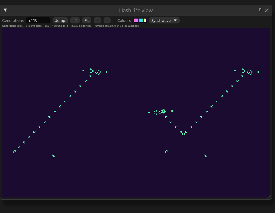
crates/jetcarp-core/data/scenes/life-not.json) after 210 generations, in the
Synthwave palette. Drawn by the app's offscreen test (see docs/tools/render-figures.sh).What HashLife can run
- Tilings: any periodic tiling. Each unit cell of the tiling is one site of HashLife’s lattice, holding the states of all its tiles, so the square grid (with either neighbourhood), hexagons, the Archimedean and k-uniform tilings, the isohedral types and the editable families all work. The aperiodic Penrose, hat and spectre tilings have no lattice, so they do not.
- Rules: those whose next state depends only on a cell’s own state and how many neighbours are in state 1: Life-like rules and Generations rules (rules with B0 included), WireWorld and Greenberg–Hastings. A world may have several such automata, on shared or separate fields. Any other rule is refused by name.
- Ages are not kept. After a jump every live cell has age 1, so age colouring starts over, and the
world’s state hash differs from that of a world stepped the same distance even though every cell
matches. Compare the hash of the cell states alone:
w.states_hash()in a script,cells_hashin the world status, or--compareon the command line. - Limits: jumps of up to 262 generations, and up to 65,536 different states per site (the number of states raised to the number of tile types in the unit cell). Memory is kept in check by a cap on the number of stored blocks (48 million by default, about 2 GB), beyond which unused blocks are cleared out; that never changes the result.
Two ways to jump
On the unbounded plane. The world’s live cells are taken out of their grid and run on an infinite plane, ignoring the grid’s edges, and the result is brought back as a new world: by default the same frame as the original, or any region of the plane. This works for any qualifying world on a periodic tiling.
In place, on a torus. A world with wrapped edges whose width and height, in unit cells, are both
powers of two (such as 256 × 128) is a torus that HashLife can advance exactly as stepping would. The
jump is logged as a jump command, so the scene replays it. A world with dead or live edges, or with a
sequence installed, cannot be jumped in place.
In the app
Run → Jump opens a small menu with a Generations box, which takes a number or a form such as
2^40 or 1e6, and three choices:
- Jump ahead (HashLife) jumps the world in place. When the world does not qualify, the button is greyed out and hovering over it says why (for example, HashLife needs a torus whose sides are powers of two (this one is 200 × 140 unit cells)).
- On the unbounded plane shows the same frame after that many generations on the plane, as a new world named after the old one (… +1000000 (HashLife plane)).
- HashLife view… opens the pattern on the plane in a window of its own, also under Tools → HashLife view…. Opening it pauses the world.
In the HashLife view, type a number of generations and press Jump, or +1 for one more. Drag to pan and scroll to zoom about the pointer; Fit frames the whole pattern, and − and + halve and double the zoom. Colours uses the world’s palette or any other. The line under the toolbar gives the generation, the number of live sites, the pattern’s extent in unit cells and the zoom. The view draws straight from HashLife’s blocks at the level where one block is about one screen pixel, so zoomed out it is as fast after 240 generations as after 100; zoomed in, every tile is drawn in its real shape. Jumps run in the background while the window shows the last frame.
On the command line
jetcarp hashlife takes a scene, a record exported from the pattern library, or a pattern in RLE or
plaintext. A Gosper glider gun, 240 generations on:
$ jetcarp hashlife gosper.rle --gens 2^40 --png gun.png
input:      gosper.rle
mode:       plane (square B3/S23)
generation: 1099511627776 (+1099511627776 in 0.008s)
population: 183251938004 (was 36)
bounds:     i 0..274877906961, j 0..274877906948 (274877906962 × 274877906949 unit cells)
nodes:      9277 live, 9277 peak, 0 collections
region:     i0 -8, j0 -8, 274877906978 × 274877906965
png:        gun.png (1025x1025, density map)
On the plane, the options choose what to export: --region i0,j0,w,h (in unit cells), or world
for the source scene’s own frame (the default is the pattern’s bounding box plus --margin, 8), and
--boundary for the exported world’s edges. --save FILE writes the region as a new scene, which
starts at generation 0 with every cell at age 1 (it has no recorded hash, so run it with jetcarp run
rather than jetcarp verify). --png FILE draws it with JETCARP’s renderer up to --max-cells cells
(16 million) and as a density map above that, in --palette, at most --max-side pixels. --rule
overrides the rule (RLE files default to their header’s rule, else B3/S23).
--torus jumps a scene in place instead, and --compare cpu (or gpu) also runs the ordinary
engine and checks that every cell agrees:
$ jetcarp hashlife torus.json --torus --gens 5000 --compare cpu
input:      torus.json
mode:       torus (Square (parallelogram) (square): 65536 cells, 256x256 unit cells, 1 tile type(s), storage dense, edges wrap)
generation: 5000 (+5000 in 0.200s)
population: 1969
states:     730e938cfe04df96
hash:       4cd23522a2a2780b
nodes:      71640 live, 71640 peak, 0 collections
compare:    cpu (32 threads) 3.539s, states equal
Saved with --save, a torus jump keeps the jump command in the scene’s log, so jetcarp verify
replays it. --node-cap changes the number of stored blocks before a clear-out, and --leaf-level
(at most 6) how large a block is stepped directly by a fast bit-parallel stepper for Life-like and
Generations rules without B0; neither changes the result.
In a script
let w = world(#{ tiling: "square", size: [256, 256], boundary: "wrap", rng_seed: 1 });
w.add_ca("B3/S23", #{ seed: "random:0.3" });
print(w.can_jump());           // true, or the reason it cannot
w.jump("2^20");                // in place, logged as a jump command
print(w.states_hash());
let later = hashlife(w, 1000); // on the plane: a new world, same frame and edges
hashlife(w, n, #{ region: [i0, j0, w, h], boundary: "dead", node_cap: 48000000 }) chooses the region
and edges of the result; region: "fit" with margin takes the pattern’s bounding box. See
Scripting (Rhai) API.
Long runs HashLife cannot help with
HashLife needs regularity and a lattice. For everything else:
- Run headless.
jetcarp run scene.json --gens Nruns as fast as the machine allows, with no drawing, on all cores;--gpusteps on the graphics adapter where the rules allow it, with an identical result. In the app, Run → Max speed and Run → GPU simulation do the same. - Save and carry on.
jetcarp run … --saverecords where a run got to, and running the saved scene again continues from there. - Large sandpiles have their own method, which builds a pile of any size by doubling (see Large sandpiles).
- Movers on aperiodic tilings can be followed for millions of tiles on a sliding window that is built around them as they go (see Aperiodic patches and following movers).
- Searches run as resumable jobs, so they can run for days and survive restarts (see Searching for patterns).
HashLife was described by R. Wm. Gosper in “Exploiting regularities in large cellular spaces” (Gosper 1984). JETCARP claims nothing new about the algorithm itself.
Aperiodic patches and following movers
The Penrose, hat and spectre tilings never repeat, so they cannot be wrapped into a torus the way a periodic grid can. JETCARP builds finite patches of them instead, round pieces of the infinite tiling chosen by level, with dead edges. A pattern that travels across one of these tilings, a mover, soon reaches the edge of any patch. To see how far it really goes, JETCARP follows it on a sliding window: only the tiles near the live cells exist, and the window is rebuilt ahead of the pattern as it moves, so the memory needed depends on the window, not on the distance. This guide covers patches and their levels, running rules on them, and following movers.
Patches and levels
| Level | Hat, Penrose kites and darts, Penrose rhombs | Spectre |
|---|---|---|
| 1 | 10 tiles | |
| 2 | 70 | |
| 3 | 500 | 559 |
| 4 | 4,000 | 4,401 |
| 5 | 35,000 | 34,649 |
| 6 | 280,000 | 272,791 |
| 7 | 2,240,000 | 2,147,679 |
| 8 | 17,920,000 | 16,908,641 |
For the hat and both Penrose tilings, a level is a size: the given number of tiles nearest a fixed centre, so patches are round and each contains the smaller ones. For the spectre, a level is a supertile level of its substitution. Levels 7 and 8 are built in exact integer coordinates, with every neighbour found by an exact lookup; level 8 has 17 to 18 million tiles and needs more than a gigabyte of memory with its neighbour graph. Each tiling’s page in the encyclopedia says how it is built.
Patches always have dead edges: cells past the edge are missing and count as empty, so patterns near
the edge behave differently from patterns deep inside. The tiles have fixed shapes and cannot be
edited, and the number of neighbours varies from tile to tile (jetcarp tilings lists the ranges:
a spectre tile has 4 to 7 edge neighbours, a Penrose rhomb 7 to 11 touching ones).
In the app, choose the tiling under Tiling → Family (or in the Tiling pane), where the four aperiodic tilings have a group of their own, then the level under Size, which lists levels 3 to 8 with their tile counts (Level 4 (4,401 tiles)). A new aperiodic world starts at level 3. The Edges choice is greyed out.
In a scene the level is the size:
"tiling": {"family": "spectre", "size": {"level": 5}}
and in a script, world(#{ tiling: "hat", size: #{ level: 4 } }) or, for short,
world(#{ tiling: "hat", level: 4 }). Levels 1 to 8 can be used in both.
Running rules on patches
Almost every rule family runs on the aperiodic tilings; only the few tied to a grid, such as the elementary row rules and von Neumann’s automaton, do not (see How JETCARP generalises automata). The Quick Start has examples, such as B2/S34 on the hat, Sandpile on the Spectre, Spectre glider and Brian’s Brain on Penrose rhombs. Searches work on patches too: the bounded soup search runs soups on a patch, and the evolutionary glider search evolves rules that make gliders on the spectre or the hat (see Searching for patterns and Search methods). HashLife does not, since these tilings have no lattice.
When you hover over the grid in the app, the bottom left corner shows the number of the cell under the pointer and its state in each field (cell 4071 · field 0: 1). Cell numbers are the tile numbers of the patch at that level, which is how the mover commands below name starting cells.
Following a mover
A glider on an aperiodic tiling never repeats exactly, since the tiles it crosses never repeat, so it cannot be proved to run for ever by finding its period. JETCARP measures instead how far it has been seen to travel unchanged, and calls it verified to a distance: so many rings of tiles (edge steps from the starting tiles to the nearest live tile), with the distance also given in neighbour steps and in plane units. There are two ways to follow one.
On a sliding window, as a resumable job, with jetcarp search mover:
$ jetcarp search mover --rule SpectreGlider --tiling spectre --rings 200 --store
mover job 1 in /home/ada/.local/share/jetcarp/library.sqlite
start: 4071:1,4097:3
mover 1: 200 rings of 200 (634 units) after 404 of 40000 generations, 11757 gens/s, 5821 rings/s, level 7, 603 tiles | verified to distance 200 edge rings (200 touching-neighbour steps, 633.6 units) over 404 generations on a sliding window of spectre (supertile level 7, at most 1009 tiles), population 2-12; stopped at the requested distance
library: 4b70f6b289a68075
The window never held more than about a thousand tiles. This is how JETCARP followed James Edmond’s Spectre glider pair for 10 million rings of tiles, and the hat glider for a million (see Findings).
Over fixed patches of growing level, with jetcarp library movers track, which runs the pattern on
each patch from --level up to --max-level (7 on the spectre by default, where 8 is on request; the
largest elsewhere) and checks that each level agrees with the one before:
$ jetcarp library movers track --rule SpectreGlider --tiling spectre --gens 3000
start: 4071:1,4097:3
verified to distance 224 edge rings (224 touching-neighbour steps, 708.2 units) over 451 generations on spectre level 7 (2147679 tiles), population 2-12; stopped at the edge of the largest patch
  level 4 (4401 tiles): 35 generations, Edge, 16 rings, population 2-12, 0.0s
  level 5 (34649 tiles): 35 generations, Edge, 16 rings, population 2-12, agrees with the smaller level, 0.1s
  level 6 (272791 tiles): 268 generations, Edge, 132 rings, population 2-12, agrees with the smaller level, 2.0s
  level 7 (2147679 tiles): 451 generations, Edge, 224 rings, population 2-12, agrees with the smaller level, 7.2s
  group of 5 cells at 712.0 units, heading 107.9 degrees
  group of 6 cells at 712.0 units, heading -131.7 degrees
Both commands take the same description of the pattern:
| Option | Meaning |
|---|---|
--rule | The rule: SpectreGlider (the default), a priority table ("Priority 4: …") or a B/S rule |
--tiling | spectre (the default), hat, penrose-kd or penrose-rhomb |
--level | The patch level the starting cells are numbered on (default 4) |
--nb | touch (the default) or edge |
--cells | The starting cells as CELL:STATE pairs, such as 1203:1,1204:3 |
--states, --at | Instead of --cells: put these states (such as 1,3) on tile --at and its edge neighbours in order; with no --at, try pairs around the deepest tile of the patch until one travels |
--gens, --max-pop | Stop after this many generations (default 20,000; with --rings, 100 more per ring), or when the pattern grows past this many live cells (default 2,000) |
--store, --json-out | Add the mover to the pattern library once verified, with the distance; write the full report as JSON |
jetcarp search mover also takes --rings (stop, verified, at this distance), --margin (how much of
the tiling to keep around the live cells, in plane units, default 24) and --fixed-levels (on the
spectre, the window follows the same tiles as the fixed patches up to this level, default 8), and
the options every search job has: --label, --minutes, --limit, --resume, --detach,
--threads and --library (see Search methods). A run stops
when it reaches the distance asked for, the generation limit or the edge of the largest patch, or
early when the pattern dies, grows past the cell limit or repeats in place (then it is an oscillator,
not a mover).
The library keeps movers with the distance they were verified to. jetcarp library movers list lists
them, farthest first, and jetcarp library movers verify ID follows one again from where it was
stored (20,000 generations by default) and updates its record.
In a script, track_mover(#{ rule: "SpectreGlider", tiling: "spectre", level: 4, cells: [[4071, 1], [4097, 3]], window: true, rings: 100 }) does the same and returns the report; without window it
tracks over the fixed patches. library().query(#{ class: "mover" }) lists the stored movers (see
Scripting (Rhai) API).
How the window stays exact
Every tile of the window is placed by an exact rigid motion in integer coordinates, so tiles built at different times match exactly and neighbours are found without rounding. Live cells are always kept at least three neighbour steps from the window’s open edge, so every cell that can change sees its true neighbours, and the run equals the run on the whole infinite tiling. The method is described in full in Search methods.
Website export
jetcarp site export turns the public part of your library into a folder you can put on any web
host: one JSON file per pattern, ant run or Quick Start entry, its pictures and animation, a
manifest.json that lists everything, and a viewer page, index.html, that shows it all as a grid.
Run it again after curating and it writes only what changed and deletes what is no longer public, so
the folder can be synced to a host as it is.
A website export is for people to look at. To give someone data they can import, check and build on, make a pack instead.
Export
$ jetcarp site export --to site
wrote   patterns/21e9bac2df7b770a5ff0f34bd68a514a.json
wrote   media/pattern/21e9bac2df7b770a5ff0f34bd68a514a/anim.gif
wrote   media/pattern/21e9bac2df7b770a5ff0f34bd68a514a/poster.png
wrote   media/pattern/21e9bac2df7b770a5ff0f34bd68a514a/thumb.png
…
wrote   manifest.json
wrote   index.html
site: 2 patterns, 0 Quick Start entries; 10 files written, 0 deleted, 0 items unchanged, 2 media rendered
Pictures and animations a pattern doesn’t have yet are rendered first, in the house style. Use
--palette NAME (or hex colours) to render them in another palette, or --no-render to export
only the media that already exist. They are the same files jetcarp media render makes (see
Pictures and animations). --frames copies each animation’s frames as PNGs too.
Run the same command again and it compares each file’s hash with the copy already in the folder:
$ jetcarp site export --to site
site: 2 patterns, 0 Quick Start entries; 0 files written, 0 deleted, 2 items unchanged, 0 media rendered
What counts as public
Only what you’ve curated goes out. By default that is:
- patterns you’ve marked
reviewedorpromoted(jetcarp library update ID --state reviewed, or in the app’s library window); - ant and turmite runs in the same two states;
- Quick Start entries you’ve added yourself.
A rejected pattern never goes out. Mark an exported pattern rejected (or back to new), export
again, and its files are deleted from the folder.
To narrow it further:
| Option | Effect |
|---|---|
--state LIST | Pattern curation states to export, comma-separated (default promoted,reviewed) |
--class LIST | Only these classes, such as spaceship,oscillator |
--min-score X | Only patterns with at least this interest score |
--min-rating N | Only patterns you’ve rated at least N stars (1–5) |
--min-osc-period N | Leave out oscillators with a shorter period |
--ants LIST | Ant curation states to export (none for no ants) |
--ant-outcome LIST | Only ants with these outcomes, such as highway,symmetric |
--quickstart LIST | Which Quick Start entries to export (none for none) |
View it
Browsers don’t let a page read files from a file:// address, so serve the folder over HTTP to look
at it on your own computer:
$ python3 -m http.server -d site 8000
Then open http://localhost:8000/. The page shows every item’s animation in a grid, with filters by
kind and class, a sort order (highest score first by default), a search box over names, rules and
grids, and a detail view for each item.
The page is plain HTML and JavaScript with no build step and nothing loaded from elsewhere, so it
works from any static host. --no-page leaves it out, for instance if you’ve written your own
page over manifest.json. A page of your own can also read the data from another folder: the
viewer’s DATA constant, near the top of its script, names the folder that holds
manifest.json.
Put it online
Copy the folder to any static host: GitHub Pages, Netlify, an S3 bucket or your own server. Files
that haven’t changed keep their names and contents, so a sync tool such as rsync or
aws s3 sync uploads only the new ones after each export. The page asks for each file with its hash
in the address, so browsers and caches never show a stale picture.
The files
| Path | What it holds |
|---|---|
index.html | The viewer page |
manifest.json | Every item, with its kind, id, title, class, grid, rule, file path and hash, and the filter that made the export |
patterns/<id>.json | A pattern’s record: its rule and the range of rules it works in, tiling, period, displacement, cells, phases and scores |
ants/<id>.json | An ant or turmite run’s record |
quickstart/<id>.json | A Quick Start entry, with its scene |
media/<kind>/<id>/ | thumb.png, poster.png and anim.gif (and frames with --frames) |
Each JSON file has a format field (1). The page refuses nothing, but warns in the browser’s
console about a manifest format it doesn’t know.
Uninstalling
JETCARP keeps almost everything in three folders, for settings, data and output (see
Folders). Outside them it sets things up only when you ask it to: the
background host starting at login, the GNOME Shell extension, the Windows or macOS screen saver, and
a still picture as your desktop background. Removing JETCARP takes three steps: undo those with
jetcarp uninstall, decide what to do with the folders, and remove the program itself.
1. Undo what JETCARP set up
jetcarp uninstall, on its own, shows what it would do without changing anything:
$ jetcarp uninstall
Would undo (run again with --yes):
  stop the host starting at login

Kept the data folder /home/ada/.local/share/jetcarp (2.1 GB); add --data to delete it.
Your pictures and exports in /home/ada/Pictures/JETCARP are never deleted.

To remove the program itself, use what installed it: the installer again with `--uninstall`, `pipx uninstall jetcarp`, `uv tool uninstall jetcarp`, `pip uninstall jetcarp`, `brew uninstall jetcarp`, `scoop uninstall jetcarp`, `cargo uninstall jetcarp`, or delete its folder.
jetcarp uninstall --yes does it, and reports each step as done or FAILED with the reason. The
steps it may list are:
- stop the background host;
- put your own desktop picture back, if the host left a still there (Leave a still picture when
it stops, or
jetcarp host still on) or will as it stops. JETCARP saved your picture when it first put a still up; if you have chosen another picture since, that one is left alone; - stop the host starting at login;
- remove the GNOME Shell extension (Linux): it is switched off and its folder deleted. Log out and back in once to finish;
- remove the Windows screen saver (
JETCARP.scr), clearing the choice in Windows’ screen saver settings if JETCARP was the one chosen; - remove the macOS screen saver (
JETCARP.saver); - forget the recorded host command, a small file in the settings folder that GNOME’s menu and the Windows screen saver use to start the host.
Run it from your desktop session where you can, since putting your picture back and switching the GNOME extension off both go through the desktop. From another desktop, a text console or over SSH it still finds the GNOME extension’s files and deletes them; GNOME Shell skips an extension on its list whose files have gone.
Two options also delete JETCARP’s folders:
| Option | Deletes |
|---|---|
--settings | The settings folder: the app’s and the host’s settings, screensaver profiles, rotations, reseed presets you saved, and the host’s desktop pictures. A picture there that the desktop still shows is kept, and the report names it: on Windows the copy of your own picture that was put back, or a still if it could not be |
--data | The data folder: the pattern library with its media, jobs and Quick Start entries (the atlas and your own), and the exploratory search’s databases. This cannot be undone |
The output folder, with your pictures, wallpapers, script runs and sweeps, is never deleted. If you
want to keep your pattern library, copy library.sqlite (and its media folder) out of the data
folder first; jetcarp doctor shows where it is. If you moved the library elsewhere with
JETCARP_LIBRARY, --data does not delete it. Like every JETCARP command, jetcarp uninstall uses
the folders that JETCARP_CONFIG_DIR, JETCARP_DATA_DIR and JETCARP_OUT point to when they are
set; jetcarp paths shows which.
2. What lives where
If you would rather remove things by hand, or check that nothing is left, this is everything JETCARP
writes outside the program’s own folder. ~ is your home folder.
| What | Linux | macOS | Windows |
|---|---|---|---|
| Settings folder | ~/.config/jetcarp | ~/Library/Application Support/jetcarp | %APPDATA%\jetcarp |
| Data folder | ~/.local/share/jetcarp | ~/Library/Application Support/jetcarp/data | %LOCALAPPDATA%\jetcarp |
| Output folder (kept) | ~/Pictures/JETCARP | ~/Pictures/JETCARP | your Pictures folder, \JETCARP |
| Runtime files (a port number, an access token and a lock file) | $XDG_RUNTIME_DIR/jetcarp, else ~/.cache/jetcarp | ~/.cache/jetcarp | inside the data folder |
| Start at login | ~/.config/autostart/jetcarp-host.desktop | ~/Library/LaunchAgents/com.jimmieprodgers.jetcarp.host.plist | the value JETCARP under HKEY_CURRENT_USER\Software\Microsoft\Windows\CurrentVersion\Run |
| GNOME Shell extension | ~/.local/share/gnome-shell/extensions/jetcarp@jimmieprodgers.com, and its entry in GNOME’s list of enabled extensions | ||
| Screen saver | ~/Library/Screen Savers/JETCARP.saver | %LOCALAPPDATA%\JETCARP\JETCARP.scr, and the SCRNSAVE.EXE value under HKEY_CURRENT_USER\Control Panel\Desktop when it is the chosen one | |
| Screen saver log | jetcarp-saver.log in the screen saver’s sandbox (~/Library/Containers/com.apple.ScreenSaver.Engine.legacyScreenSaver/Data/tmp/ on macOS 27) |
The Linux paths are the usual ones; they follow your XDG settings. jetcarp uninstall does not remove
the runtime files or the macOS screen saver’s log, which are small; delete them by hand if you like.
To remove the GNOME extension by hand, switch it off in GNOME’s Extensions app before deleting its
folder, or run jetcarp host gnome remove, which does both.
3. Remove the program
Remove the program last: jetcarp uninstall needs it to undo the rest. Then use what installed it
(see Installing JETCARP):
| Installed with | Remove with |
|---|---|
| The shell installer | curl -LsSf https://github.com/jprodgers/jetcarp/releases/latest/download/jetcarp-installer.sh | sh -s -- --uninstall, or sh jetcarp-installer.sh --uninstall: it deletes ~/.local/lib/jetcarp and the link ~/.local/bin/jetcarp |
| The PowerShell installer | the installer again with -Uninstall: it deletes %LOCALAPPDATA%\Programs\jetcarp and takes it off your user PATH |
| pipx, uv, pip | pipx uninstall jetcarp, uv tool uninstall jetcarp, pip uninstall jetcarp |
| Homebrew | brew uninstall jetcarp (and brew untap jprodgers/jetcarp) |
| Scoop | scoop uninstall jetcarp (and scoop bucket rm jetcarp) |
| cargo | cargo uninstall jetcarp |
| A release archive | delete the folder you unpacked |
Each removes the program with the files that came with it (on Windows jetcarpw.exe, the
windowless launcher; on macOS libjetcarp_saver.dylib; the starter pack) and nothing of yours: the
settings, data and output folders stay until you delete them (step 1’s --settings and --data,
or by hand). If you built JETCARP from source, delete the folder you built it in.
How JETCARP generalises automata to any tiling
Almost every well-known cellular automaton was invented on the square grid, and most of their rules are written in terms of that grid: “the eight surrounding cells”, “the cell above”, “turn left”. JETCARP runs these rules on hexagons, pentagons, mixtures of polygons, tiles you draw yourself and aperiodic tilings such as the hat. It can do this because it reduces every tiling to the same object, a neighbour graph, and rewrites each rule family in terms of that graph. This page explains the graph, the choices it involves, and which families could not be carried over.
docs/scenes/automata/generalising-touch.json and
generalising-edge.json, 1 generation.What it is
A cellular automaton is a grid of cells, each in one of a few states, updated all at once in steps called generations. Each cell’s next state depends only on its own state and the states of its neighbours. Change what counts as a neighbour and you change the automaton.
On a tiling, the natural neighbours of a tile are the tiles next to it. JETCARP records them as a graph: one node per tile, and a link between two tiles that are neighbours. Everything a rule needs is then a question about the graph: how many neighbours are alive, which neighbour lies to the left, how far away a tile is.
There are two ways for tiles to be “next to” each other, and JETCARP offers both:
- Touch neighbours share an edge or at least one corner. On the square grid this is the eight-cell Moore neighbourhood used by Conway’s Life.
- Edge neighbours share a stretch of edge. On the square grid this is the four-cell von Neumann neighbourhood.
On squares the two give 8 and 4 neighbours. Elsewhere the numbers change, sometimes a lot. A triangle has 12 touch neighbours but only 3 edge neighbours; a Cairo pentagon has 7 and 5; a hexagon has 6 either way, because hexagons never meet at a corner alone. In a tiling with several kinds of tile, the counts differ from tile to tile: in the 4.8.8 tiling a square has 4 neighbours and an octagon 8. On aperiodic tilings they vary irregularly: a Penrose rhomb touches between 7 and 11 others. The tiling catalogue lists the counts for every tiling.
This matters because most rules count neighbours. Life’s rule “born with exactly 3 live neighbours” means something quite different when a cell has 12 neighbours, or when some cells have 4 and others 8. Much of what is interesting about running old rules on new tilings comes from this.
Where it came from
The two square-grid neighbourhoods are named after Edward F. Moore, who described machine models of self-reproduction at a 1961 symposium (Moore 1962), and John von Neumann, whose 29-state automaton used the four edge neighbours (von Neumann 1966; see LifeWiki: Moore neighbourhood and Von Neumann neighbourhood).
Running automata on other grids is almost as old. Marcel Golay used hexagonal cellular logic for image processing (Golay 1969). Carter Bays explored Life-like rules on the triangular tiling (Bays 1994) and on hexagons and pentagons (Bays 2005). Life on Penrose tilings was studied by Hill, Stepney and Wan (2005) and by Owens and Stepney (2010), and Adam Goucher found a glider that travels across a Penrose tiling (Goucher 2012). Ants and turmites have run on triangular and hexagonal grids in Tim Hutton’s Golly rules (Hutton 2015) and on Penrose tilings (ptiles/ant).
General tools came later. Ready, from the GollyGang project, runs user-defined rules on polygonal and polyhedral meshes (Ready). Andrew Trevorrow’s HatLife ran Life-like, Larger than Life-style and WireWorld rules on the hat tiling within weeks of its discovery (Trevorrow 2023), and James Edmond’s work on the hat and spectre runs Generations and priority-table rules on a general graph (Edmond 2026). In October 2026 Trevorrow’s SpectreLife did for the spectre what HatLife did for the hat, with Edmond’s rules (Trevorrow 2026), and bellissimogiorno’s aperiodic-life package runs Life on square, hexagonal and aperiodic tilings (bellissimogiorno 2026). JETCARP builds on all of this.
How JETCARP runs it
One graph, three ways of storing it
Every tiling becomes a neighbour graph in which each tile’s neighbours are kept in clockwise order. How the graph is stored depends on the tiling, but the rules never see the difference:
- Dense storage for lattices of one tile shape (squares, hexagons, bricks), where the neighbours follow a fixed stencil.
- Periodic storage for tilings that repeat a unit cell containing several tiles (the Archimedean, k-uniform and isohedral tilings, and tiles you draw), with one table of neighbour offsets per tile in the cell.
- Explicit storage for finite patches of aperiodic tilings (Penrose, hat and spectre), with every tile’s neighbour list written out.
Periodic worlds can have dead edges (cells beyond the edge count as empty), wrapped edges (a torus), or live edges (cells beyond the edge count as alive). Aperiodic patches have dead edges.
Rules that count
Life-like rules, Generations, JACA, WireWorld and the cyclic, Greenberg–Hastings,
rock-paper-scissors, Hodgepodge and forest-fire families all depend on how many neighbours are in
some state. They carry over directly: a cell counts its neighbours in the graph, whatever their
number. Each automaton in a scene chooses touch or edge; in B/S notation a trailing V means
edge neighbours, as on LifeWiki. Because some tiles have more than nine neighbours, counts of 10 or
more are written with commas: B3,10/S2,3.
The Abelian sandpile is the clearest case of a rule that depends on degree: a tile topples when it holds as many grains as it has neighbours, so on the spectre the threshold differs from tile to tile.
Rules that turn
Langton’s ant and the turmites need direction: “turn right and step forward”. JETCARP
measures turns in slots of a tile’s clockwise list of edge neighbours. R and L turn one slot
either way, U turns half the tile’s degree, and R2 and L2 turn two slots (120 degrees on a
hexagon). After a step the ant faces “straight on”, the slot opposite the edge it came in by. On a
tile with an odd number of sides there is no exact opposite, so “straight on” is rounded and stays
relative to the entry edge. This one convention lets the same ant run on squares, pentagons, mixed
tilings and the hat.
Rules that measure distance
Some families need “within r cells” or “the next row out”. JETCARP uses distance in the graph, counted in steps from neighbour to neighbour:
- Larger than Life counts the cells within
rsteps, over touch neighbours for its Moore form and over edge neighbours for its von Neumann form. On the square grid these are the usual box and diamond. - Layered rules grow outward from a seed tile one layer at a time, where a layer is all the tiles at the same graph distance. This is how JETCARP carries Wolfram’s row-by-row rules to any tiling.
- JACA’s blast radius destroys every cell within
Nsteps of an annihilation. - Lenia is the exception: its smooth kernel uses straight-line distance between tile centres, measured in units of the average tile size.
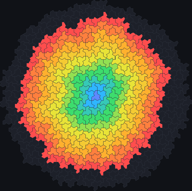
GH 14/1) starts
at one tile and advances one step of the touch neighbour graph per generation, leaving a trail of
refractory states, so each colour band is one distance from the centre. Scene
docs/scenes/automata/generalising-layers.json, 9 generations.What stays on its own grid
A few families are tied to a grid’s geometry in a way that has no natural meaning elsewhere, and JETCARP does not pretend otherwise:
- Elementary rules (
W30) read the three cells above in a square grid; the hexagonal row rules (HexW,HexT) read the hexagons above. Their any-tiling counterpart is the layered family. - Margolus block rules update 2 × 2 blocks of squares on alternating offsets.
- Von Neumann’s 29-state automaton depends on the four compass directions; JETCARP refuses to place it on another tiling.
What is new here
None of the ingredients on this page is new on its own, as the history above shows: Ready runs arbitrary rules on meshes, HatLife, SpectreLife and Edmond’s work run several families on the hat and spectre, and many single families have been run on hexagons, triangles or Penrose tilings. What JETCARP adds, to our knowledge, is breadth: one engine that runs every family listed here on every class of tiling it supports (lattices, the 1,248 k-uniform tilings, 81 isohedral types, drawn tiles, and the Penrose, hat and spectre tilings), with the same neighbour model throughout. Not all of these are different graphs: the 81 isohedral types have only the eleven graphs of the Laves tilings, and several drawn families copy the square or hexagonal grid (see Isohedral tilings). Tests check that results agree across thread counts and, where available, between CPU and GPU.
Our prior-art search found no earlier version of the cyclic, Greenberg–Hastings, rock-paper-scissors, Hodgepodge or forest-fire rules on aperiodic tilings, or of turmites on the hat and spectre. Each of these is a direct application of a known rule to a known graph, though, so we do not count them as discoveries. The search behind these statements is summarised in What is new in JETCARP.
Try it
- In the app, any Quick Start entry can be moved to another tiling: change the tiling and the rule keeps running. The Tiling showcase entries pair each tiling with a rule chosen to stay lively there.
- Run the figures above from their scenes, for example
jetcarp run docs/scenes/automata/generalising-touch.json --gens 1 --png touch.png. jetcarp tilingslists every tiling family with its edge and touch neighbour counts.
References
- Moore 1962; von Neumann 1966
- Golay 1969; Bays 1994; Bays 2005
- Hill, Stepney and Wan 2005; Owens and Stepney 2010; Goucher 2012
- Hutton 2015; ptiles/ant
- Ready; Trevorrow 2023; Edmond 2026; Trevorrow 2026; bellissimogiorno 2026
Life-like rules
Conway’s Game of Life is the best-known cellular automaton, and it belongs to a large family of rules that work the same way: each cell is alive or dead, and whether it is alive next generation depends only on whether it is alive now and how many of its neighbours are. JETCARP runs every rule of this family on every tiling it supports, with either of two neighbourhoods.

B3/S23) for 500 generations after a random start on a wrapped
128 × 80 grid (the first generations are shown more slowly). Watch the soup thin out within a few
dozen generations into islands of activity that settle one by one. Colour shows how long a cell has
been alive, as in LifeViewer's age colouring
([LifeWiki: LifeViewer](../research/bibliography.md#lifewikind_lifeviewer)): pale cells are new, deep
blue ones have not changed for a long time (still lifes such as blocks and beehives). Scene
docs/scenes/automata/life-square.json.What it is
A Life-like rule is fixed by two lists of neighbour counts:
- Birth (B): a dead cell becomes alive if its number of live neighbours is in this list.
- Survival (S): a live cell stays alive if its number of live neighbours is in this list. Otherwise it dies.
Life itself is B3/S23: a dead cell with exactly three live neighbours is born, and a live cell
with two or three survives. From these two lines come gliders that travel across the grid, guns that
fire them, and, as Conway sketched and later builders made explicit, machines that can compute
anything a computer can.

docs/scenes/automata/life-glider.json, 80 generations.Rules of this kind are called outer totalistic: the new state depends on the cell itself and the total of its neighbours, not on which neighbours are alive. On the square grid with the eight surrounding cells as neighbours, counts run from 0 to 8, so there are 218 = 262,144 Life-like rules (LifeWiki: Life-like cellular automaton). Many have names and their own communities of explorers; JETCARP’s named rule catalogue lists 96 of them.
Where it came from
Life. John Horton Conway’s Game of Life reached the public through Martin Gardner’s “Mathematical Games” column in Scientific American in October 1970 (Gardner 1970), followed by a second column in February 1971 (Gardner 1971). Conway was simplifying ideas from von Neumann’s self-reproducing automaton, and offered a $50 prize for a pattern that grows without limit; an MIT group led by Bill Gosper won it in November 1970 with the glider gun (LifeWiki: Conway’s Game of Life). Berlekamp, Conway and Guy’s Winning Ways for your Mathematical Plays (1982) gave Conway’s sketch that Life can hold a universal computer (Berlekamp, Conway and Guy 1982), and Paul Rendell later built an explicit Turing machine in Life (Rendell 2002).
Neighbourhoods. The eight-cell neighbourhood is named after Edward F. Moore (Moore 1962) and the four-cell one after John von Neumann, whose 29-state automaton used it (LifeWiki: Von Neumann neighbourhood).
The rule space. Norman Packard and Stephen Wolfram surveyed two-dimensional automata, numbering outer-totalistic rules and studying their behaviour (Packard and Wolfram 1985). David Eppstein later classified Life-like rules by whether patterns can grow out of a bounding box and whether they can die out (Eppstein 2010).
Notation. Two orders are in use. The older survival/birth form writes Life as 23/3; it was
common for years, and Mirek Wójtowicz’s MCell rule lexicon uses it
(Wójtowicz, rules lexicon). The birth/survival form
B3/S23 is the one Golly and LifeWiki use today
(LifeWiki: Rulestring). We found no source that
says who first wrote rules as B…/S….
Variants. People began trying other counts almost at once. LifeWiki traces 3-4 Life (B34/S34)
to Robert Wainwright’s newsletter Lifeline in December 1971
(LifeWiki: 3-4 Life). A few of the many named rules
that followed, with credits as the sources give them:
- HighLife (
B36/S23), first considered by Nathan Thompson in 1994 and named by Conway; it has a small replicator (LifeWiki: HighLife). - Day & Night (
B3678/S34678), explored by Nathan Thompson from 1997; swapping live and dead cells leaves it unchanged (LifeWiki: Day & Night). - Seeds (
B2/S), first studied by Brian Silverman and named by Wójtowicz (LifeWiki: Seeds). - Life without Death (
B3/S012345678), which Tommaso Toffoli and Norman Margolus described as INKSPOT (Toffoli and Margolus 1987). - Vote and Anneal, Gérard Vichniac’s majority and twisted-majority rules (Vichniac 1986).
Software. Golly, by Andrew Trevorrow and Tom Rokicki, first released in 2005, made these rules easy to explore and fast to run (Golly credits; Golly changes). Before it came the CAM-6 hardware of Toffoli and Margolus (1987), Rudy Rucker and John Walker’s CelLab (1989) and Wójtowicz’s MCell. Chris Rowett’s LifeViewer now shows patterns in the browser on LifeWiki and the forums, colouring cells by age if asked (Rowett: LifeViewer; LifeWiki: LifeViewer; Rowett 2019).
How JETCARP runs it
Notation
JETCARP reads the birth/survival form, in upper or lower case:
| Notation | Meaning |
|---|---|
B3/S23 | Life: born on 3, survives on 2 or 3, touch neighbours |
B36/S23 | HighLife |
B2/S34H | Hexagonal Life: the H records that the rule is meant for hexagons (forum thread, 2016) |
B1/S0V | Gnarl on edge neighbours: born with one live neighbour, survives with none |
B3,10/S2,3 | Counts of 10 or more are separated by commas |
B014/S2 | Oils, a rule with birth on 0 (see below) |
Any of the named rules can be typed by name instead.
Any tiling, two neighbourhoods
A Life-like rule needs only a neighbour count, so it runs unchanged on any neighbour graph (see How JETCARP generalises automata). By default a cell counts its touch neighbours, which share an edge or a corner; on squares that is Moore’s eight.
Edge neighbours: the V suffix
A trailing V switches the rule to edge neighbours, which share a side; on squares that is von
Neumann’s four. This follows LifeWiki’s convention
(LifeWiki: Rulestring). The neighbourhood can
also be set per automaton in a scene ("neighborhood": "edge").
Counts mean different things on different tilings. A triangle has 12 touch neighbours, a hexagon in the 3.3.3.3.6 tiling has 18, and a square in 4.8.8 has only 4. A rule tuned for one tiling is usually a different creature on another.
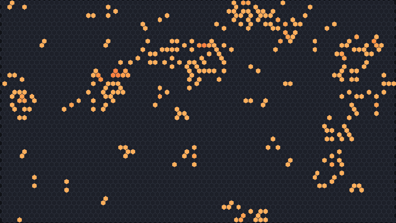
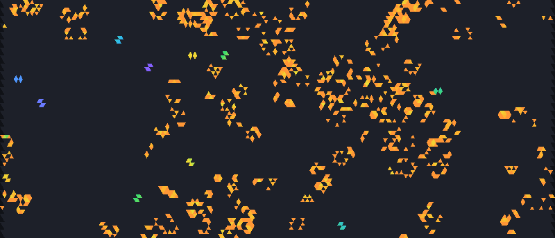
B2/S34H), 60 generations from a random start; every
hexagon has six neighbours. It has spaceships of its own, which wildmyron posted in the forum thread
that named the rule ([drc, Hickerson and wildmyron 2016](../research/bibliography.md#drc2016b2s34h)).
Scene docs/scenes/automata/life-hex.json. Right: Life's own
rule B3/S23 on triangles with touch neighbours, where each cell has twelve neighbours,
300 generations. Scene docs/scenes/automata/life-triangle.json.B0 rules
If 0 is in the birth list, every dead cell with no live neighbours is born, so the empty background switches on. Without survival on the maximum count it switches off again next generation, and the whole picture flashes. Golly avoids this by running such a rule as two complementary rules that alternate on even and odd generations, so that what you see is the rule’s real behaviour without the strobing (Golly: QuickLife); Golly credits David Eppstein with the idea (Golly credits). JETCARP does the same, and its tests check the result against running the rule by brute force. B0 rules also run under HashLife.
Speed
On lattice tilings JETCARP can step Life-like rules on the GPU as well as the CPU, with identical results, and HashLife can jump wrap-edge lattice worlds far ahead.
What is new here
Life-like rules on other tilings are not new: Carter Bays studied them on triangles, hexagons and pentagons (Bays 1994; Bays 2005), Life has been run on Penrose tilings (Hill, Stepney and Wan 2005; Owens and Stepney 2010) and on the hat (Trevorrow 2023), and H. S. Guttesen studied Life on the Archimedean tilings (Guttesen 2026).
What JETCARP adds is a search for spaceships (patterns that move) across many tilings and rules at once. Some of what it found was already known. Guttesen reported a period-4 glider and a glider gun for Life on the kagome tiling (3.6.3.6) and a period-8 glider on the snub square tiling; JETCARP’s soup searches found the same kagome glider (cell for cell, in one of its phases) and, by comparison with Guttesen’s figure, the same snub-square glider independently, and the credit for them is Guttesen’s.
Beyond those, JETCARP’s catalogue holds spaceships in Life-like rules on the 4.8.8, 3.12.12, 4.6.12, 3.4.6.4, 3.3.3.4.4 and 3.3.3.3.6 tilings, on 3.6.3.6 in rules other than Life, and on several 2- and 3-uniform tilings. Each ship was checked in three ways before it was claimed:
- Against every Archimedean, 2-uniform, 3-uniform and isohedral tiling, with both neighbourhoods. A ship that sees exactly the same neighbour counts in a corridor of a simpler tiling belongs to that tiling, and so does one whose live tiles evolve the same way there in some rule.
- For being two smaller ships flying together.
- On large patches, with wrapped edges and with dead edges.
Ten catalogue entries turned out to be pairs of smaller ships flying side by side, eight of them two of Guttesen’s kagome gliders, and they are not claimed; every Life candidate on the kagome tiling was such a pair. Eight ships found on 3-uniform tilings run unchanged on a simpler tiling, and they are listed there. A looser test, which asks only that the live tiles evolve the same way whatever the neighbour counts of the empty tiles around them, found two more catalogue entries that are the same ship as another, and eight ships that run on a simpler tiling than the one they were found on. That leaves 60 distinct objects. Thirteen are a smaller ship with a passenger, or a bound pair, and are listed with the smaller ship. Twenty-eight, six of those thirteen among them, carry a flag: they are small and turn up often in soups, run in a well-known rule, are built on Guttesen’s gliders, or run on 4.8.8 or 3.12.12 in the rules where EricG reported many unlisted spaceships in 2013 (EricG 2013), so others may well have seen them, although we found no report. To our knowledge, the remaining 25 single ships, on 3.4.6.4, 3.3.3.4.4, 3.3.3.3.6 and on 2- and 3-uniform tilings, have not been reported before. Spaceships on these tilings are not new as such: EricG found ships in Life-like rules on every Archimedean tiling, and Martin Büttner found one in Life on a 2-uniform tiling in 2014 (Code Golf 2014); only these particular ships are claimed. Only two of the 60 run in Life itself: both are on the snub square tiling, both are built around Guttesen’s glider, and both are flagged. The rest are in other rules.
The searches behind those 60 ran Life itself on only a few tilings, though. A census of Life on all 92 Archimedean, 2-uniform and 3-uniform tilings, 50,000 random soups on each, found Life spaceships on 28 of them: Conway’s glider and spaceships on the square grid, Guttesen’s two gliders, a ship on 3.3.3.4.4 that is probably the one EricG reported in 2013, the period-20 ship on k2-007 that is very likely Büttner’s, and ships on 5 of the 2-uniform and 19 of the 3-uniform tilings. To our knowledge, nobody had reported running Life on any of those 2- and 3-uniform tilings but k2-007. Most of the census’s ships are common ships flying in pairs, or ships of a simpler tiling running in a corridor; those that passed every check are listed in Life on the Archimedean and k-uniform tilings.
Ships found on isohedral tilings are not claimed at all. Each isohedral tiling has the neighbour graph of one of the eleven Laves tilings, and every “ship” JETCARP found on one is a known ship of the square or triangular grid in another drawing, Conway’s glider among them. The full list, with every check, is in Findings; the claims are on What is new in JETCARP.
Try it
- Quick Start: Life on the square grid, Life on the 12-neighbour triangle grid, B2/S34 on the hat, and one entry for every named rule, each on its usual grid.
- From the command line:
jetcarp run docs/scenes/automata/life-square.json --gens 500 --png life.png. - Change the tiling of any Life-like entry in the app and watch the same rule on a new graph.
References
- Gardner 1970; Gardner 1971; Berlekamp, Conway and Guy 1982; Rendell 2002
- Moore 1962; Packard and Wolfram 1985; Eppstein 2010
- Toffoli and Margolus 1987; Vichniac 1986; Rucker and Walker 1989
- Golly: QuickLife; Golly credits; Golly changes; Rowett 2019
- Bays 1994; Bays 2005; Hill, Stepney and Wan 2005; Owens and Stepney 2010; Trevorrow 2023; Guttesen 2026
- LifeWiki: Life-like cellular automaton, Rulestring, Conway’s Game of Life, 3-4 Life, HighLife, Day & Night, Seeds
Generations
A Generations rule is a Life-like rule in which dying cells do not vanish at once. They fade through a fixed number of “ageing” states first, and while they fade nothing can be born in their place. That one change turns static Life-like worlds into restless ones full of waves, trails and fast-moving gliders.

B2/S/C3), the first 80 generations after a random start, one
generation per frame, in part of a wrapped 160 × 100 grid. Watch the soup sort itself within a few
dozen generations into gliders: each is a front of firing cells (orange) followed by refractory ones
(blue), and they travel in straight lines until they collide. Scene
docs/scenes/automata/generations-brain.json.What it is
A Generations rule has three parts: birth counts, survival counts, and a number of states C.
- State 0 is empty and state 1 is alive. Only state-1 cells count as live neighbours.
- An empty cell is born (becomes 1) when its number of live neighbours is in the birth list.
- A live cell stays at 1 when its count is in the survival list. Otherwise it starts to age: it
moves to state 2, then 3, and so on up to
C − 1, one step per generation, and then becomes empty. - An ageing cell ignores its neighbours, and no cell can be born on top of it.
With C = 2 there are no ageing states and the rule is an ordinary Life-like rule. The ageing
states act as a wake: a pattern cannot fall back into the space it has just left, which is why so
many Generations rules are full of spaceships.
The best-known example is Brian’s Brain, B2/S/C3, which reads naturally as a model of
neurons. Each cell is ready (0), firing (1) or refractory (2). A ready cell fires when
exactly two of its neighbours are firing; a firing cell always becomes refractory (the survival
list is empty); a refractory cell becomes ready again.
Where it came from
The earliest dated member of the family we found is Brian’s Brain. Tommaso Toffoli and Norman Margolus describe it in Cellular Automata Machines (1987), in a section on the firing of neurons, as a three-state rule they ran on their CAM-6 hardware as BRIAN’S-BRAIN; a footnote says the rule was suggested by Brian Silverman, while the neuron interpretation is theirs (Toffoli and Margolus 1987). LifeWiki dates the rule to the mid-1990s (LifeWiki: Brian’s Brain), but the 1987 book shows it was published by then. Rudy Rucker and John Walker’s CelLab (Autodesk, 1989) included it as “Brain”, along with many other multi-state rules (Rucker and Walker 1989; CelLab rules).
The family got its name and its notation from Mirek Wójtowicz’s MCell (“Mirek’s Cellebration”), a
Windows program Wójtowicz began in January 1999
(Wójtowicz 2024). MCell made Generations a named
family with a survival/birth/states notation, and its documentation calls it perhaps the most
beautiful family in the program (MCell families).
We found no source that says who first used the name. Wójtowicz’s own Star Wars (B2/S345/C4)
dates from March 1999 (LifeWiki: List of Generations rules).
Around MCell grew a community of rule authors. The MCell rules lexicon and LifeWiki’s list credit rules to Wójtowicz, John Elliott, Michael Sweney, Charles A. Rockafellor, Scott Robert Ladd, Brian Prentice, Jason Rampe, Anders Starmark, Rudy Rucker and John Walker, and others (MCell rules lexicon; LifeWiki list); the named rule catalogue gives the credit for each rule. Golly added Generations in version 2.0 in December 2008 (Golly changes; Golly: Generations).

B2/S345/C4) from generation 40 to 120 after a random
start, one generation per frame. Live cells survive with three to five neighbours and fade through two
dying states; watch small ships fly off while the debris decays behind them. Scene
docs/scenes/automata/generations-starwars.json.How JETCARP runs it
Notation
JETCARP writes Generations rules as LifeWiki does, B…/S…/C<states>, with 2 to 255 states:
| Notation | Rule |
|---|---|
B2/S/C3 | Brian’s Brain |
B2/S345/C4 | Star Wars |
B2/S/C3V | Brian’s Brain on edge neighbours |
B3/S23/C2 | Two states: the same as Life, B3/S23 |
B2/S/3 (no C) is also accepted. MCell’s survival/birth order is not; write the birth list
first. Forty-five named Generations rules can be typed by name (see the
catalogue).
On any tiling
Like Life-like rules, Generations rules only count live neighbours, so they run on every tiling’s
neighbour graph with touch neighbours by default, or edge neighbours with the V suffix (see
How JETCARP generalises automata). Brian’s Brain on Penrose rhombs, below, keeps
its waves going across a tiling with no repeating pattern at all.

docs/scenes/automata/generations-penrose.json.Colours, speed and long runs
Each state gets its own colour from the palette. On lattice tilings Generations rules can be stepped on the GPU with identical results, and HashLife can jump wrap-edge lattice worlds far ahead, including rules with birth on 0.
What is new here
Nothing on this page is new. Generations-style rules have run on the hat in Andrew Trevorrow’s HatLife (Trevorrow 2023) and on the hat and spectre in James Edmond’s work (Edmond 2026). JETCARP’s part is running the family on every tiling it supports with the same engine as everything else.
Try it
- Quick Start: Brian’s Brain, Brian’s Brain on Penrose rhombs, and one entry for each of the 45 named Generations rules.
jetcarp run docs/scenes/automata/generations-brain.json --gens 200 --png brain.png- Try Brian’s Brain with edge neighbours (
B2/S/C3V) on the hat; with fewer neighbours, firing needs a different count to spread.
References
- Toffoli and Margolus 1987; Rucker and Walker 1989; CelLab rules
- Wójtowicz 2024; MCell families; MCell rules lexicon
- LifeWiki: Generations, List of Generations rules, Brian’s Brain
- Golly: Generations; Golly changes
- Trevorrow 2023; Edmond 2026
Larger than Life
Larger than Life widens Life’s neighbourhood. Instead of the eight cells around it, a cell looks
at every cell within some range r, and is born or survives when the number of live cells there
falls in a range of values. With a large enough neighbourhood, Life’s small, jagged creatures give
way to big, smooth, almost organic ones.

R5,C2,S33-57,B34-45), 300 generations after a random start on a
wrapped 200 × 125 grid. Each cell counts the live cells in the 11 × 11 box around it. Watch the soup
die back within a few generations, leaving hollow blobs that wobble, merge and break up; the small
ones that keep their shape and travel are the "bugs" the rule is known for. Scene
docs/scenes/automata/ltl-bosco.json.What it is
A Larger than Life rule has a range r, a neighbourhood shape, and a birth and
survival condition given as ranges of counts:
- On the square grid, the usual (Moore) shape is the box of side
2r + 1around the cell, so a range-5 cell has 120 neighbours. The von Neumann shape is the diamond of cells withinrsteps up, down, left and right. - A dead cell is born when the number of live cells in its neighbourhood is in the birth range; a live cell survives when the count is in the survival range.
Life is the range-1 case. Larger ranges average over more cells, which smooths out the randomness of small counts: patterns grow round edges and move as large coherent bodies. Kellie Evans showed that rescaled versions of Life’s gliders and replicators exist at large ranges; Evans called the gliders “bugs” (Evans 1996).
The modern generalisation, higher-range outer-totalistic (HROT) rules, allows any list of counts rather than a single interval for birth and for survival (LifeWiki: HROT).
Where it came from
Golly’s documentation credits David Griffeath with first imagining Larger than Life in the early 1990s, to see whether Life sits near a critical point when its thresholds and range are scaled up together (Golly: Larger than Life). Golly cites Griffeath’s “Self-organization of random cellular automata: four snapshots” as the first reference (Griffeath 1994).
Kellie Michele Evans developed the family in a 1996 PhD thesis at the University of Wisconsin–Madison, Larger than Life: It’s So Nonlinear, supervised by Griffeath. Evans’s preface says the question came from Griffeath: would glider-like “digital creatures” emerge from random starts if Life’s rule were rescaled to larger neighbourhoods? The thesis studies the family with tools from probability and from dynamics, including large-range analogues of Life’s replicators and gliders (Evans 1996). Evans continued the work in a series of papers (Evans 2001; Evans 2003; Evans 2003, replicators; Evans 2005; Evans 2010; Evans 2016).
MCell’s rules lexicon says the “Bugs” rule was found while exploring the parameter space on the CAM-8 cellular automaton machine, and credits it to Evans (MCell rules lexicon). Golly’s help says that “Bosco”, a period-166 oscillator, was discovered by Evans, and that Dean Hickerson used MCell to build the first bug gun from it (Golly: Larger than Life). The rule became known as Bosco’s Rule (LifeWiki: Larger than Life). Other named rules include Griffeath’s Majority, Majorly and Bugsmovie, Evans’s Waffle, Wójtowicz’s Globe and Charles A. Rockafellor’s ModernArt (see the catalogue).
Mirek Wójtowicz’s MCell (from 1999) gave the family its first widely used notation, with ranges up to 10 (MCell families). Chris Rowett’s LifeViewer added Larger than Life and HROT rules in January 2019, accepting Adam P. Goucher’s lifelib notation for HROT (Rowett 2019). Golly added a Larger than Life algorithm in version 3.0 (2017) and HROT rules in 4.0 (2020) (Golly changes).
How JETCARP runs it
Notation
JETCARP reads both the HROT form and MCell’s form:
| Notation | Meaning |
|---|---|
R5,C2,S33-57,B34-45 | Bosco’s Rule in HROT form: range 5, two states, survival on 33 to 57, birth on 34 to 45 |
R5,C0,M1,S34..58,B34..45,NM | The same rule in MCell’s form, where M1 counts the cell itself, so the survival bounds are one higher |
R2,C2,S4-8,B5-7,NN | The von Neumann (diamond) shape |
R3,C2,S2,B3,N+ | Factorio, on the cross-shaped neighbourhood (square grid only) |
R10,C255,S1-2,B3 | ModernArt: with more than two states, dying cells decay as in Generations |
In HROT form the centre cell is never counted. Counts can be lists of values and ranges separated
by commas. Rules with weighted or custom neighbourhoods (an NW… suffix) are not supported yet,
so the named rule Coexistence cannot be run.
On any tiling
On the square grid the Moore shape is the box and the von Neumann shape the diamond. On any other
tiling JETCARP measures range in steps over the neighbour graph: Moore means “within r steps over
touch neighbours” and von Neumann means “within r steps over edge neighbours”. On the square grid
these definitions give exactly the box and the diamond, and range 1 is checked to equal Life. The
cross shape has no such reading and stays on the square grid.
Neighbourhood sizes change with the tiling, so a rule’s thresholds usually need adjusting when it moves. On the hat, below, Bosco’s thresholds are scaled down by a quarter, and bug-like hollow blobs appear on an aperiodic tiling.

R5,C2,S25-43,B26-34): the neighbourhood is every
tile within five steps of the touch neighbour graph. The middle of a patch of about 4,000 hats, 300
generations from a random start; watch the soup clump into blobs whose edges shift and smooth
themselves over the irregular tiles. Scene docs/scenes/automata/ltl-hat.json.What is new here
Larger than Life-style range rules have run on the hat before, in Andrew Trevorrow’s HatLife (Trevorrow 2023); we did not confirm whether HatLife measures range in graph steps. Golly supports hexagonal, triangular and other neighbourhood shapes (Golly: Larger than Life). We do not claim anything new for this family. Defining range as graph distance is what lets JETCARP run the family on every tiling, including the k-uniform, isohedral and aperiodic ones.
Try it
- Quick Start: the eight runnable named rules, for example Bosco’s Rule, Majority (LtL) and ModernArt.
jetcarp run docs/scenes/automata/ltl-bosco.json --gens 300 --png bosco.png- Move Bosco’s Rule to hexagons and lower its thresholds until bugs appear; the neighbourhood of range 5 is smaller there than on squares.
References
- Griffeath 1994; Evans 1996; Evans 2001; Evans 2003; Evans 2003, replicators; Evans 2005; Evans 2010; Evans 2016
- MCell rules lexicon; MCell families
- Golly: Larger than Life; Golly changes; Rowett 2019
- LifeWiki: Larger than Life, Higher-range outer-totalistic
- Trevorrow 2023
Elementary (Wolfram) rules
The elementary cellular automata are the simplest interesting ones: a single row of cells, each alive or dead, where each cell’s next state depends on itself and its two neighbours. There are only 256 such rules, yet among them are rules that make nested fractals, rules that look random, and one that can compute anything. JETCARP draws them the classic way, one row per generation down the square grid.
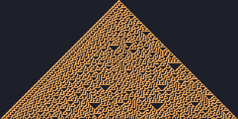
W30) from a single live cell. Each row is one generation, computed from
the row above. Scene docs/scenes/automata/elementary-rule30.json, run until the bottom
row is written.What it is
A cell and its two neighbours form a pattern of three cells, and there are eight possible patterns (from 111 down to 000). An elementary rule says which of the eight patterns produce a live cell in the next generation. Reading those eight outputs as a binary number, from pattern 111 down to 000, gives the rule’s number between 0 and 255. Rule 30 is 00011110 in binary: patterns 100, 011, 010 and 001 produce a live cell, the rest a dead one.
Because the automaton is one-dimensional, its whole history fits in one picture: put each generation below the last. Some famous members:
- Rule 90, where each cell is the exclusive or (XOR) of its two neighbours. From one cell it draws Pascal’s triangle mod 2, the Sierpinski triangle.
- Rule 30, whose centre column looks random enough to be used as a source of pseudorandom bits.
- Rule 110, in which moving structures collide on a periodic background, and which can emulate any computer.
- Rule 184, where live cells move right when the cell ahead is empty: a simple model of traffic.
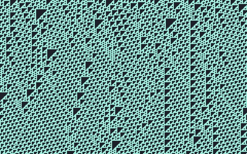
W110) from a random first row on a wrapped grid. Scene
docs/scenes/automata/elementary-rule110.json.Where it came from
One-dimensional cellular automata were studied in symbolic dynamics as maps that commute with the shift; Gustav Hedlund’s 1969 paper is the standard reference for that line of work (Hedlund 1969).
Stephen Wolfram studied the 256 three-neighbour rules systematically in “Statistical mechanics of cellular automata” (1983), numbering each rule by its outputs read as a binary number, the scheme now called the Wolfram code (Wolfram 1983; Wikipedia: Wolfram code). In 1984 Wolfram sorted cellular automaton behaviour into four qualitative classes, from rules that die out to rules with complex, long-lived structures (Wolfram 1984), and with Olivier Martin and Andrew Odlyzko worked out the algebra of the additive rules such as 90 and 150 (Martin, Odlyzko and Wolfram 1984). Wolfram proposed rule 30 as a random-number generator in 1986 (Wolfram 1986).
Wolfram’s 1985 list of open problems asked which cellular automata are computation-universal (Wolfram 1985). Matthew Cook proved that rule 110 is, by showing it can emulate cyclic tag systems. Cook presented the proof at the CA98 conference at the Santa Fe Institute; Wolfram Research then took legal action over Cook’s nondisclosure agreement, and the proof was published in 2004 (Cook 2004; Wikipedia: Rule 110; Giles 2002). Turlough Neary and Damien Woods later showed that rule 110 simulates Turing machines efficiently, so predicting it is P-complete (Neary and Woods 2006). Wolfram’s A New Kind of Science (2002) brought the elementary rules to a wide audience (Wolfram 2002).
How JETCARP runs it
Notation
| Notation | Rule |
|---|---|
W30 | Rule 30 (Rule 30 also works) |
W90 | Rule 90 |
W110 | Rule 110 |
W0 to W255 | Every elementary rule, odd numbers included |
Golly’s Wn rules are limited to even numbers, because in an odd rule the empty pattern 000
produces a live cell, which raises the same problem as B0 rules
(Golly: QuickLife). JETCARP runs odd rules too: their
background simply alternates from row to row, which shows as stripes.
Rows on the square grid
An elementary rule in JETCARP fills the square grid from the top down: each generation computes the
next row from the one above it. The first row is set by the seed: one live cell in the middle
(top_center) or a random row (top_random). With dead edges, cells beyond the sides count as dead;
with wrapped edges the row is a ring, and the rule keeps going for one full pass of the grid. The
run is done when the bottom row has been written, which searches and scripts use to know when to
stop. Colour by row gives the gradients often seen in pictures of these rules.
An elementary rule can share a field with other automata: in the Quick Start entry Rule 30 meets Life and ants, Life rewrites the rows rule 30 leaves behind while ants wander through them.
Not on other tilings
“The cell to the left and the cell to the right in the row above” only makes sense on a grid with
rows, so the W rules stay on squares. JETCARP carries the idea elsewhere in two ways: the
hexagonal row rules, which read the two or three hexagons above a cell, and
layered rules, which replace rows with layers of graph distance and run on any tiling.
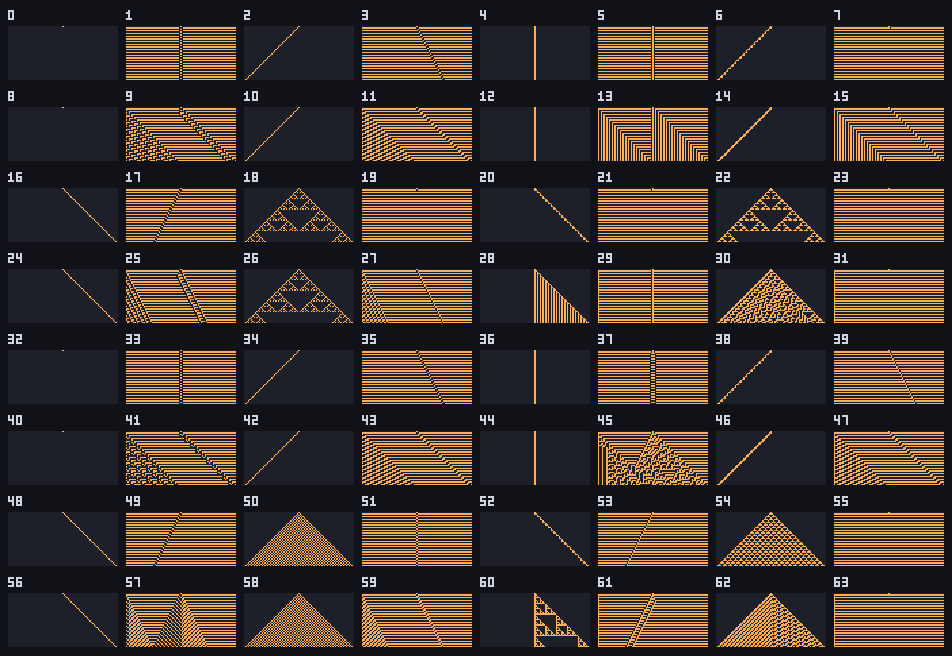
jetcarp sheet --kind w --from 0 --count 64. Odd rules turn the empty background on and
off, which shows as stripes.What is new here
Nothing. The elementary rules are among the most studied objects in the field, and JETCARP runs them as everyone does. Its own additions are the hexagonal and layered families described on their own pages.
Try it
- Quick Start: Rule 30, Rule 90, Rule 110, and ten more named rules (18, 22, 45, 54, 60, 73, 105, 126, 150, 184).
jetcarp sheet --kind w --from 64 --count 64 --png sheet.pngdraws the next 64 rules.jetcarp run docs/scenes/automata/elementary-rule110.json --gens 200 --png rule110.png
References
- Hedlund 1969
- Wolfram 1983; Wolfram 1984; Martin, Odlyzko and Wolfram 1984; Wolfram 1985; Wolfram 1986; Wolfram 2002
- Cook 2004; Giles 2002; Neary and Woods 2006
- Wikipedia: Wolfram code, Rule 110, Rule 184
- Golly: QuickLife
Hexagonal row rules: HexW and HexT
Elementary rules build a picture row by row on the square grid, each cell reading the three cells
above it. On a grid of hexagons the rows are staggered, so a cell sits under two cells, or, if
the hexagons are turned to have flat tops, under three cells at two different heights. JETCARP has
a family for each: HexW with two parents and HexT with three. Both come in binary and
three-state versions.
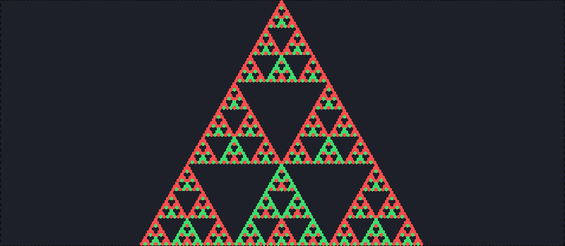
HexW3 8229 from a single cell: each hexagon is the sum, mod 3, of the two
hexagons above it, which draws Pascal's triangle mod 3. Red and green are the two non-zero states.
Scene docs/scenes/automata/hex-hexw3.json, run until the bottom row is written.What it is
Two parents (HexW, HexW3). On a grid of pointy-topped hexagons, each hexagon touches two
hexagons in the row above, one up and to the left, one up and to the right. A two-parent rule gives
the new cell’s state as a function of those two. With two states there are 2 × 2 = 4 parent
patterns and so 24 = 16 rules; with three states there are 9 patterns and
39 = 19,683 rules. HexW 6 is the exclusive or of the two parents, which draws Pascal’s
triangle mod 2 just as rule 90 does on squares.
Three parents (HexT, HexT3). Turn the hexagons a quarter turn so they have flat tops. Now
three hexagons touch a cell’s upper edges: NW and NE, half a row higher, and N, a full row higher.
The grid fills in by height in half-row layers, and each new layer is computed from the two layers
before it. With two states there are 8 parent patterns and 256 rules, numbered like Wolfram’s
elementary rules; with three states there are 27 patterns and 327 (about 7.6 trillion)
rules. Two smaller sets are easier to explore: totalistic rules, which depend only on the sum
NW + N + NE (2,187 three-state rules, 16 binary ones), and left-right symmetric rules, which treat
NW and NE alike.
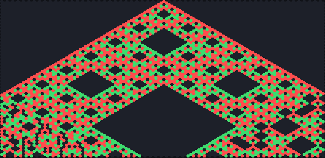
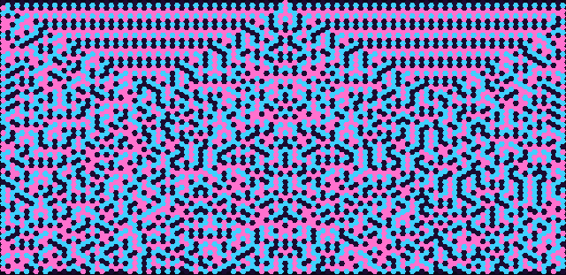
HexT3 sum 588, NW + N + NE mod 3, grows nested diamonds. Right: HexT3 sum 314
turns chaotic. Scenes docs/scenes/automata/hex-hext3-sum588.json and
hex-hext3-sum314.json, run until the bottom layer is written.Where it came from
Hexagonal grids have a long history in cellular automata. Marcel Golay used hexagonal cellular logic for image processing in 1969 (Golay 1969). Norman Packard and Stephen Wolfram’s survey of two-dimensional automata counted the rules on the hexagonal neighbourhood alongside the square ones (Packard and Wolfram 1985), and the hexagonal lattice gas of Frisch, Hasslacher and Pomeau showed why hexagons matter for physics: their symmetry is enough to recover fluid flow, where the square grid’s is not (Frisch, Hasslacher and Pomeau 1986).
The two-parent rules are Wolfram’s. In a note in A New Kind of Science, Wolfram observes that
if the cells on successive steps are arranged “like hexagons or staggered bricks”, each cell depends
on two cells instead of three; Wolfram counts 16 two-colour rules and 19,683 three-colour rules, of which
1,734 are fundamentally different (Wolfram 2002, p. 885).
HexW and HexW3 are exactly this family. Matej Kerekrety’s 2020 web tool also draws the 16 binary
rules on hexagons, along with the 256 elementary rules on squares and pentagons
(Kerekrety 2020).
The three-parent rules are a known kind of rule in a new presentation. A cell that depends on
two cells one layer back and one cell two layers back is a second-order one-dimensional automaton
on a staggered lattice. Second-order rules are standard: A New Kind of Science uses them to build
reversible rules (p. 437 and the note on p. 1017), and the Wolfram Language’s CellularAutomaton
supports staggered ranges and rules of any order
(Wolfram 2002;
Wolfram Language documentation). The 16
HexT rules of the form g(NW, NE) XOR N are exactly the reversible second-order versions of the 16
two-parent rules.
How JETCARP runs it
Notation
| Notation | Family | Rule number |
|---|---|---|
HexW 6 | two parents, 2 states | 0 to 15; the output for parents (left, right) is digit left·2 + right of the number in base 2 |
HexW3 8229 | two parents, 3 states | 0 to 19,682; digit left·3 + right in base 3 |
HexT 90 | three parents, 2 states | 0 to 255; bit NW·4 + N·2 + NE |
HexT3 n | three parents, 3 states | 0 to 327 − 1; digit NW·9 + N·3 + NE in base 3 |
HexT3 sum 588 | three parents, 3 states, totalistic | 0 to 2,186; digit NW + N + NE in base 3 |
HexT sum 6 | three parents, 2 states, totalistic | 0 to 15 |
HexT3 sym n | three parents, 3 states, symmetric | 0 to 318 − 1 |
HexT 90 is NW XOR NE, Pascal’s triangle mod 2 again; HexT 150 is the XOR of all three parents;
HexT 4 copies N straight down.
Grids
The two-parent rules run on the ordinary hexagon tiling (hex). The three-parent rules need the
flat-top hexagon tiling (hex_flat), whose rows are the half-row layers. As with the
elementary rules, each generation writes one more row or layer from a seed at the
top (top_center for one cell, top_random for a random row), with dead, live or wrapped edges, and
the run is done when the bottom is reached. These families are tied to rows of hexagons and do not
run on other tilings; the any-tiling version of the idea is the layered family.
Sheets and sweeps
jetcarp sheet --kind hexw, hexw3, hext, hext3 or hext3sum draws a contact sheet of
consecutive rules, and scripts can sweep whole sets. A first run classified all 256 HexT rules and
all 2,187 HexT3 sum rules from a single cell with JETCARP’s row descriptors, which label the rows a
rule leaves behind as uniform, periodic, shifting or aperiodic (and the aperiodic ones as nested,
regular or chaotic). For HexT that gave 44 uniform, 127 periodic, 46 shifting and 39 aperiodic
rules, three of them chaotic (153, 165 and 195). The labels are a quick heuristic, not a proof.

HexW 0 to HexW 15, from a single cell:
jetcarp sheet --kind hexw --count 16.What is new here
The two-parent rules are not new: they are Wolfram’s two-cell rules, drawn on hexagons as Wolfram describes, and Kerekrety’s tool draws the binary ones too.
The three-parent rules are built from standard ingredients, but we found no earlier source that
presents them as a family of hexagon rules, numbers all 256 binary and 327 three-state
rules in this way, adds the totalistic and symmetric subsets, or catalogues them. To our knowledge,
presenting and cataloguing the HexT and HexT3 family is new with JETCARP. The search behind this
is summarised in What is new in JETCARP.
Try it
- Quick Start: Hex rule 6 (XOR), Hex ternary 8229 (sum mod 3), Hex3 rule 90 (NW xor NE), Hex3
ternary sum 588 (sum mod 3) and Hex3 ternary sum 314. On a hexagon rule’s card,
<and>step through the rule numbers. jetcarp sheet --kind hext3sum --from 0 --count 64 --png sheet.pngdraws 64 totalistic three-parent rules.jetcarp run docs/scenes/automata/hex-hext3-sum588.json --gens 200 --png diamonds.png
References
- Wolfram 2002 (p. 885 note on two-cell neighbourhoods; p. 437 and the p. 1017 note on second-order rules); Wolfram Language: CellularAutomaton
- Kerekrety 2020
- Golay 1969; Packard and Wolfram 1985; Frisch, Hasslacher and Pomeau 1986
Layered rules
A layered rule is an elementary-style rule that grows outward from a seed instead of downward from a top row. The “rows” are the layers of the tiling’s neighbour graph around the seed: the seed, then every tile next to it, then every tile next to those, and so on. Because any tiling has layers in this sense, the same rule runs on squares, Cairo pentagons and the aperiodic spectre alike.
Layer 2/01 grown from one tile of a patch of about 35,000 spectres: each tile in a
new layer is the parity of its parents. Coloured by position from top to bottom. Scene
docs/scenes/automata/layered-spectre.json, run until the last layer is written.What it is
Pick one or more seed tiles. The layers are the sets of tiles at the same distance from the seeds, counting steps from neighbour to neighbour: layer 0 is the seeds, layer 1 the tiles that touch them, and so on. Each generation writes the next layer.
A tile’s parents are its neighbours in the layer before. A layered rule is totalistic: the
new tile’s state depends only on the sum of its parents’ states. The rule is a list of outputs,
one for each sum, and the list repeats, so the output for sum s is entry s mod the list’s length:
Layer 2/01: two states; an even sum gives 0 and an odd sum gives 1. Each tile is the parity (XOR) of its parents.Layer 3/012: three states; each tile is the sum of its parents mod 3.
The totalistic form is what makes this work on any tiling. On squares every cell has the same number of parents, but on a Cairo or spectre tiling the number of parents varies from tile to tile, and a rule that depends only on the sum stays well defined.
On the square grid with edge neighbours the layers are diamonds, and Layer 2/01 draws Pascal’s
triangle mod 2 in each quarter, the same pattern rule 90 draws from one cell
(Martin, Odlyzko and Wolfram 1984). On other
tilings the same rule draws patterns that have no simple formula.
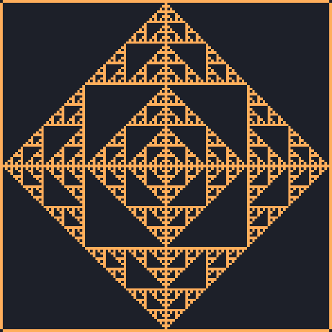
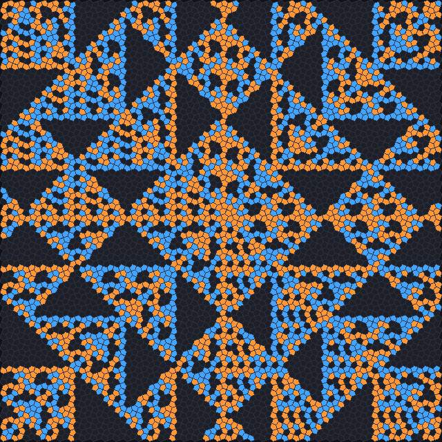
Layer 2/01 on squares with edge neighbours, grown from the centre; the
layers are diamonds and each quarter holds Pascal's triangle mod 2. Scene
docs/scenes/automata/layered-square.json. Right: Layer 3/012 on Cairo
pentagons with edge neighbours, the sum of the parents mod 3. Scene
docs/scenes/automata/layered-cairo.json. Both run until the last layer is written.Where it came from
Layered rules are Jimmie Rodgers’s construction, introduced in JETCARP in 2026. They combine the row-by-row picture of Wolfram’s one-dimensional rules (Wolfram 1983) with a tiling’s neighbour graph.
The closest earlier work we found carries one-dimensional rules into other tilings in different ways. Maurice Margenstern embedded one-dimensional automata in hyperbolic tilings along a chosen line of tiles (Margenstern 2010), and Matej Kerekrety’s web tool draws elementary rules row by row on hexagons and pentagons, using the lattice’s fixed rows (Kerekrety 2020). Neither uses graph-distance layers from a seed.
A note on the name: Abhishek Dalai’s “Layered Cellular Automata” (Dalai 2023) is a different idea, two coupled layers of computation, and is unrelated to JETCARP’s layered rules.
How JETCARP runs it
Notation
Layer <states>/<outputs>, where the outputs are listed for sums 0, 1, 2, … and repeat:
| Notation | Rule |
|---|---|
Layer 2/01 | Parity: rule 90 grown on any tiling |
Layer 3/012 | Sum mod 3: Pascal’s triangle mod 3 on any tiling |
Layer 2/0110 | Output 1 for sums 1 and 2, 0 for sums 0 and 3, repeating every four |
Seeds, neighbours and edges
The layers are computed once, by a breadth-first search over the automaton’s neighbourhood (touch or edge), from every cell that is non-zero when the rule first runs. With no live cells it starts from the centre tile and switches it on. Several seeds give layers that grow from all of them at once and meet in the middle. The run is done when the last layer has been written; on a finite patch that is when the layers reach its edge.
Touch and edge neighbourhoods give different layers. On squares, touch layers are square rings and edge layers are diamonds; on most other tilings the two differ in more irregular ways, and so do the pictures.
Colour
By default each tile is coloured by state. Colour by row ("color_by": "row") shades tiles by
their height in the picture instead, as in the spectre figure above.
What is new here
To our knowledge, layered rules are a new presentation: Wolfram-style totalistic rules whose rows are the graph-distance shells around a seed, so that they run unchanged on any tiling, including aperiodic ones. We found no earlier source that defines them or runs them on Penrose, hat or spectre tilings. The idea is simple enough that it may exist unpublished, for example in hobby code or in work on rules over graphs that our search did not reach, so we claim only that we have not seen it published. The search is described in What is new in JETCARP.
Try it
- Quick Start: Layered parity on the Spectre, Layered parity and Layered sum mod 3 (both on Cairo pentagons).
jetcarp run docs/scenes/automata/layered-spectre.json --gens 400 --png spectre-layers.png- Seed a few cells by hand with the Draw tool before starting a layered rule: the layers then grow from all of them.
References
- Wolfram 1983; Martin, Odlyzko and Wolfram 1984
- Margenstern 2010; Kerekrety 2020
- Dalai 2023 (unrelated, same name)
JACA: Jimmie’s Annihilating Cellular Automata
JACA is a family of two-sided Life-like rules. Cells are positive, negative or empty; each sign grows by its own birth/survival rule; and wherever the two signs touch, they destroy each other. Started from a mixed soup, the two signs sort themselves into territories separated by glowing, shifting fronts, and the fight between them can last thousands of generations. JACA is Jimmie Rodgers’s idea and is introduced in JETCARP.

JACA B27/S03456 on Cairo pentagons, 1,500 generations after a mixed start (the
early generations are shown more slowly). Watch the two signs sort themselves into territories: inside
them nothing changes, so cells grow old and take the last colour of their palette, while along the
fronts cells keep being destroyed and reborn, so age colouring turns each front into a rainbow. Scene
docs/scenes/automata/jaca-cairo-rainbow.json (Quick Start preset JACA rainbow fronts
(Cairo)).What it is
Each cell holds one of three values: +1, −1 or 0 (empty), a balanced ternary digit. Every generation is computed from the current state in three steps:
- Contact. A live cell with at least one neighbour of the opposite sign is a contact cell. Contact cells are destroyed: they are empty next generation.
- Blast. With a blast radius
Ngreater than 0, every cell withinNneighbourhood steps of a contact cell is destroyed too, whatever its sign. With the defaultblast 0, only the touching cells go. - Everything else follows its own sign’s rule. A +1 cell survives if its number of +1 neighbours is in the +1 rule’s survival list; an empty cell is born +1 if its number of +1 neighbours is in the +1 rule’s birth list; and likewise for −1. Each sign counts only neighbours of its own sign. An empty cell that both signs would fill stays empty: the two births cancel.
Two properties make the family easy to reason about. A world that contains only one sign runs that
sign’s plain birth/survival rule exactly, so JACA B3/S23 with only +1 cells is Conway’s Life.
And the two signs can follow different rules: JACA +B3/S23 -B36/S23 sets Life against HighLife.
What emerges depends on the rules, the tiling and the blast radius. Among the behaviours found so far:
- Territory wars. Seeds-like rules (birth on 2, little survival) in mixed soups form territories that merge and push along their fronts until one sign holds the whole grid, on every tiling tried.
- Rainbow fronts. In rules whose territories go still while their fronts stay active, colouring by age turns every front into a rainbow, as in the figure above.
- Trenches. A blast radius of 1 to 3 leaves a strip of no-man’s-land between territories: bands, beads, ropes, collapsing loops.
- Annealing. With births on 3 or more, fronts become smooth and move to reduce their curvature, like grain boundaries in a cooling metal.
- Two different rules. Bubbles of one rule growing in the other’s still sea, or still crystal against noise, with either side winning.


JACA B27/S013), 1,500 generations, seen
where two armies meet; watch the front, marked by grey and pale destroyed tiles, push back and forth.
Scene docs/scenes/automata/jaca-hat-war.json. Right: blast radius 1 on squares
(JACA B16/S1378 blast 1), 1,500 generations: the borders between the signs are bands of
destroyed, glowing cells; watch them straighten and the territories trade ground. Scene
docs/scenes/automata/jaca-square-beads.json. Both are Quick Start presets.Where it came from
JACA is Jimmie Rodgers’s idea, from November 2026; it first appeared in JETCARP’s predecessor CART on 8 November 2026. Each of its ingredients has a precedent, and we credit them here:
- Two-player Life. Mark Levene and George Roussos’s two-player game of life (2003) has black and white tokens; opponents weaken each other’s survival through a difference count, and a tie at birth is settled by a coin flip (Levene and Roussos 2003).
- +1, −1 and 0, with cancelled births. The CodinGame bot game “Game of Life or Death”, described on the Unsupervision Blog in November 2025, encodes the two players as 1 and −1; each side treats the other’s cells as dead, and a cell both sides would switch on stays dead (Unsupervision Blog 2025). This is the closest precedent for JACA’s encoding, own-sign counting and cancelled births. Touching cells of opposite sides are not destroyed there.
- Matter and antimatter Life. In September 2018 KittyTac proposed, on the ConwayLife.com forums, a Life with two kinds of cell where contact turns both cells into energy, and wildmyron implemented it as the “Energetic” rule, in which the energy decays into photons (KittyTac and wildmyron 2018; LifeWiki: Rule:Energetic). This is the closest precedent for annihilation on contact. There the products are part of the state and can create cells, and both kinds follow one fixed rule.
- Physics. Opposite particles that annihilate when they meet, A + B → 0, are a classic problem in the physics of diffusion (Toussaint and Wilczek 1983); Chopard and Droz treat such reaction–diffusion processes with cellular automata (Chopard and Droz 1998).
How JETCARP runs it
Notation
| Notation | Meaning |
|---|---|
JACA B3/S23 | Both signs follow Life |
JACA +B3/S23 -B36/S23 | +1 follows Life, −1 follows HighLife |
JACA B3/S23 blast 2 | Life for both, and each annihilation clears everything within two steps |
JACA B13/S234V | V on a B/S part: edge neighbours instead of touch neighbours |
The blast radius runs from 0 to 64. Rules with birth on 0 are refused. Counts of 10 or more are written with commas, as in other B/S rules.
On any tiling
JACA uses only neighbour counts and neighbourhood steps, so it runs on every tiling (see How JETCARP generalises automata); the blast radius is measured in steps of the automaton’s own neighbourhood. It runs on the CPU; there is no GPU or HashLife version yet.
Seeds, colours and counts
A JACA field is stored as a three-state field (states 1 and 2 are +1 and −1), so drawing, scenes
and scripts treat it like any other multi-state rule. The usual start is a mixed soup
({"signed": {"density": 0.3, "negative": 0.5}}: 30% of cells live, half of them negative); a
halves start puts +1 cells on the left and −1 on the right. Each sign has its own palette
(palette and palette_neg), coloured by age. Destroyed cells glow briefly and fade; the glow is
drawn only and is not part of the state or its hash. The app’s card shows the number of cells of each
sign and how many were touching and destroyed; the world status that scripts and the MCP server read
also reports cancelled births.
Presets
The Quick Start’s JACA family has 5 named rules and 71 presets. Each preset is a whole scene: tiling, neighbourhood, a rule per sign, blast radius, start and palette pair. Together they cover 24 tilings, from squares and hexagons through the Archimedean and k-uniform tilings to two isohedral tilings, both Penrose tilings, the hat and the spectre. (For a rule, the isohedral IH28 is the Cairo tiling and IH41 the square grid, and the brick, herringbone and Pythagorean presets play on the hexagonal, hexagonal and 4.8.8 graphs; see Isohedral tilings.) They came from a six-hour search over about 130,000 configurations: random rule pairs, mutations and crossovers of the best, and transplants of good pairs to other tilings, scored on balance between the signs, contact along fronts, territory changing hands and activity, then reviewed by eye as contact sheets.
What is new here
Each ingredient of JACA has been published before, as the list above shows, and we do not claim “the first signed Life” or “the first matter–antimatter Life”. To our knowledge, JACA’s particular combination is new: an independent birth/survival rule for each sign, counting only same-sign neighbours; destruction of every live cell that touches the other sign; a blast radius measured in neighbourhood steps; cancelled double births; an exact reduction to the plain rule when one sign is alone; and all of this on any periodic or aperiodic tiling. The searches behind this statement, and their known gaps (MCell’s weighted rules and parts of the ConwayLife forums were not searched), are described in What is new in JETCARP.
The colouring is not part of the claim: colouring cells by age and fading destroyed cells have precedents in other programs.
Try it
- Quick Start, family JACA: JACA Life, JACA Life vs HighLife, JACA war on the hat tiling, JACA rainbow fronts (Cairo), JACA bead borders (square, blast 1), and the other presets.
jetcarp run docs/scenes/automata/jaca-hat-war.json --gens 3000 --png hat-war.png- Try a halves start with two different rules, and watch which front advances.
References
- Levene and Roussos 2003
- Unsupervision Blog 2025
- KittyTac and wildmyron 2018; LifeWiki: Rule:Energetic
- Toussaint and Wilczek 1983; Chopard and Droz 1998
Langton’s ant and turmites
Langton’s ant is a single moving agent with a two-line rule: on a white cell turn right, on a black cell turn left; flip the colour of the cell and step forward. From an empty grid it wanders for about ten thousand steps in what looks like chaos, then suddenly starts building a straight “highway” and never stops. Turmites generalise the ant to more colours and to internal states. JETCARP runs them on any tiling.

Ant RL) on an empty grid, about 12,000 steps at 150 steps a frame. For
about ten thousand steps it builds an irregular, roughly symmetric blob; then, quite suddenly, it
starts the diagonal highway that repeats every 104 steps and leaves the blob for good. The red cell is
the ant. Scene docs/scenes/automata/turmite-langton.json.What it is
An ant sits on a cell, facing one of the cell’s sides. Each step it reads the colour of its cell,
turns according to that colour, changes the cell to the next colour, and moves to the neighbour it
now faces. A turn string gives the turn for each colour: Langton’s ant is RL (two colours: right
on colour 0, left on colour 1), and LLRR has four colours, each cell cycling through 0, 1, 2, 3.
A turmite adds internal states: what it writes, how it turns and which state it moves to all depend on both its state and the cell’s colour, like a Turing machine whose tape is the plane. An ant is a turmite with one state.
These agents are interesting for how much they do with so little. The RL ant’s highway repeats every
104 steps, moving two cells diagonally each period. Some turn strings, such as LLRR, grow patterns
that keep returning to perfect mirror symmetry; others fill squares or triangles, or wander forever.
A single ant can compute: its path can be made to evaluate any logical circuit.


LLRR over 120,000 steps; watch its blob grow and
keep returning to mirror symmetry. Scene docs/scenes/automata/turmite-llrr.json. Right:
Langton's ant on Cairo pentagons over 30,000 steps, here without a highway; the pentagons' outlines
show the tiling under the cloud. Scene docs/scenes/automata/turmite-cairo.json.
RNL (turn right, go on, or turn left, by the colour of the
tile) on the trihexagonal tiling 3.6.3.6, about 3,000 steps. After roughly 2,600 steps of disorder it
builds a highway that repeats every 36 steps and runs straight out of the picture. One of 39,744
highways on non-square tilings in JETCARP's catalogue, all re-verified on the release engine. Scene
docs/scenes/automata/turmite-trihex-highway.json.Where it came from
Christopher G. Langton described single-state two-dimensional Turing machines, which Langton called vants (virtual ants), in “Studying artificial life with cellular automata” (1986); the RL ant is among them (Langton 1986). Greg Turk’s 2025 review credits Langton with the term and, as far as Turk knows, with being the first to study such machines. Turk also points to a related earlier idea, the “worms” of Paterson and Conway that Martin Gardner wrote about in 1973 (Turk 2025; Gardner 1973).
Turk rediscovered the RL ant independently and sent several two-dimensional Turing machines to A. K. Dewdney, whose Scientific American column of September 1989 presented them and coined the name tur-mite (Dewdney 1989; Turk 2025). David Gale’s columns in The Mathematical Intelligencer took up the ant (Gale 1993) and reported James Propp’s work on ants whose turns are a string of Ls and Rs (Propp 1994). Gale, Propp, Scott Sutherland and Serge Troubetzkoy identified a class of ants whose patterns are, at times, bilaterally symmetric, and proved it (Gale et al. 1995); the columns were collected in Gale’s Tracking the Automatic Ant (Gale 1998). Ian Stewart’s 1994 Scientific American article brought the ant to a wide audience (Stewart 1994).
Physicists met the same dynamics independently, as a particle bouncing off rotators that flip when hit, a Lorentz lattice gas. Bunimovich and Troubetzkoy’s recurrence results are the source usually cited for the theorem that the ant’s path is always unbounded (Bunimovich and Troubetzkoy 1992); Kong and Cohen studied related lattice gases on the triangular lattice (Kong and Cohen 1991). Gajardo, Moreira and Goles showed that the ant’s path can compute any boolean circuit, so predicting it is P-hard (Gajardo, Moreira and Goles 2002), and Tsukiji and Hagiwara extended hardness results to generalised ants on square and hexagonal grids (Tsukiji and Hagiwara 2011).
The highway’s onset is usually given as step 9,977, with period 104 (Hutton 2015); we have not traced that number to a primary publication, but JETCARP’s own run reproduces it exactly. Tim Hutton’s Golly scripts generate turmite rules, including on triangular and hexagonal grids, and Hutton’s page credits Allen H. Brady with first studying the triangular case (Hutton 2015). Other programs that run ants include CelLab (Rucker and Walker 1989), Uri Wilensky’s NetLogo model (Wilensky 2005) and, on Penrose tilings, ptiles/ant (ptiles/ant). Turk’s 2025 paper publishes much of Turk’s own work from around 1989, including multistate, universal and self-reproducing turmites (Turk 2025).
How JETCARP runs it
Notation
| Notation | Meaning |
|---|---|
Ant RL | Langton’s ant |
Turmite LLRR | Four colours, one state |
Turmite RL2NU | Turns for hexagons: R, L2 (two slots), N (none), U (U-turn) |
Turmite 1R1,1L0/1R1,0N0 | A table: two states (separated by /) and two colours (separated by ,) |
In a table each entry is <colour to write><turn><next state>, one group per state and one entry per
colour. Up to 16 colours and 16 states are allowed, with 10 to 15 written a to f.
Turns on any tiling
A turn is counted in slots of the current tile’s edge neighbours, listed clockwise. R and L
turn one slot, R2 and L2 two slots (120 degrees on a hexagon), U half the tile’s number of
sides, and N not at all. After a step, the ant faces “straight on”: the side opposite the one it
came in by. A tile with an odd number of sides has no opposite side, so straight on is rounded, and
on such tiles N and U are relative to the entry edge. With this one convention the same turn
string runs on squares, hexagons, pentagons, mixed tilings and the aperiodic tilings, even though
R means 90 degrees on a square, 60 on a hexagon and something irregular on a hat (see
How JETCARP generalises automata).
Running and searching
In a scene, an ant automaton takes steps_per_gen (how many ant steps make one generation) and an
ants seed with a count; several ants can share a field, and on a field shared with other automata
they interact with Life or an elementary rule. At a dead edge an ant either bounces or falls off.
For research, jetcarp search ants runs turn strings and turmite tables on an unbounded periodic
tiling and classifies every run. When it reports a highway, it has proved one: it checks that the ant and
every cell ahead of it recur, shifted, after a fixed number of steps, which by induction repeats
forever. It reproduces the RL ant’s published highway (period 104, onset 9,977) and finds, for
example, a highway for LNL on hexagons with period 35 from step 161,093. This engine is tested to
agree cell for cell with the ordinary world’s turmites on seven tilings.
What is new here
Ants have run on hexagons, triangles and Penrose tilings before (see above). Our prior-art search found no earlier turmites on the hat or spectre tilings, but that is a direct application of a known rule to a known graph, so we do not count it as a discovery. We make no novelty claim for this family.
Try it
- Quick Start: Langton’s ant, Four-colour turmite LLRR, and the named turmites RLR, LRRRRRLLR, LLRRRLRLRLLR and RRLLLRLLLRRR.
jetcarp run docs/scenes/automata/turmite-langton.json --gens 120 --png ant.png- Move Langton’s ant to the hat or to 4.8.8, where tiles of different degree make
Rmean different angles from step to step.
References
- Langton 1986; Turk 2025; Gardner 1973; Dewdney 1989
- Gale 1993; Propp 1994; Gale et al. 1995; Gale 1998; Stewart 1994
- Bunimovich and Troubetzkoy 1992; Kong and Cohen 1991; Gajardo, Moreira and Goles 2002; Tsukiji and Hagiwara 2011
- Hutton 2015; Rucker and Walker 1989; Wilensky 2005; ptiles/ant
WireWorld
WireWorld is a cellular automaton for building circuits. You draw wires, and “electrons” run along them, split at junctions, and are stopped or passed by small arrangements of wire that act as diodes and logic gates. With enough wire it can compute anything; David Moore and Mark Owen, with help from others, built a complete programmable computer in it (Moore and Owen: The Wireworld computer).

docs/scenes/automata/wireworld-adder.json.What it is
Each cell is in one of four states: empty, conductor (copper), electron head or electron tail. The rule:
- An empty cell stays empty.
- An electron head becomes an electron tail.
- An electron tail becomes conductor.
- A conductor cell becomes an electron head if exactly one or two of its neighbours are electron heads; otherwise it stays conductor.
A head followed by its tail is an electron with a direction: the tail behind it stops it moving backwards. The “one or two” condition is what makes the circuits work. Where wires meet, a junction shaped so that an electron coming one way sees one head and one coming the other way sees three can pass electrons in only one direction (a diode), and similar small shapes give OR, AND, XOR and NOT gates, clocks and memory (LifeWiki: WireWorld).
Where it came from
WireWorld was devised by Brian Silverman, who also created Brian’s Brain and Seeds. LifeWiki says Silverman proposed it in 1987 as part of the program Phantom Fish Tank (LifeWiki: WireWorld), and the CelLab manual’s references list The Phantom Fishtank (Logo Computer Systems, Montreal, 1987) (Silverman 1987). A 2025 blog post gives 1984 instead (daneelsan 2025), so the rule itself may be older than the program; we have not been able to settle this.
A. K. Dewdney’s Scientific American column of January 1990 described WireWorld and made it widely known (Dewdney 1990; LifeWiki: WireWorld). David Moore and Mark Owen, “with the help of many others”, designed a complete programmable computer in WireWorld between 1990 and 1992 and wrote it up in September 2004 (Moore and Owen: The Wireworld computer); a copy that computes prime numbers ships with Golly (LifeWiki: WireWorld). WireWorld has long been built into MCell and Golly, and Andrew Trevorrow’s HatLife ran it on the hat tiling in 2023 (Trevorrow 2023).
How JETCARP runs it
Notation and states
The rule is written WireWorld. States are 0 (empty), 1 (electron head), 2 (electron tail) and 3
(conductor), drawn by default as dark background, blue, red and amber; use the Draw tool to paint
wire and electrons.
On any tiling
WireWorld only asks how many neighbours are electron heads, so it runs on any neighbour graph (see How JETCARP generalises automata). The circuits designed for the square grid depend on its geometry, though: a junction that is a diode on squares is just a blob of wire on hexagons. On another tiling you have to find new gates, which is part of the fun. Touch neighbours are the default, as in the classic rule; edge neighbours make thin wires behave differently at corners. WireWorld can be stepped on the GPU on lattice tilings, and HashLife can jump wrap-edge lattice worlds far ahead.
The adder
The adder in the figure was built for JETCARP, cell by cell, by code that can regenerate and check
it. Every component keeps one timing rule: electrons that leave their sources together reach each
column together, so the inputs of every gate arrive at the same moment and no delay lines are
needed. Its parts are fan-outs, a three-cell OR junction and a 17-cell XOR junction in which two
simultaneous electrons annihilate. The OR and XOR junctions were found by JETCARP’s own search, an
exhaustive scan of small junction shapes and simulated annealing, not copied from earlier designs.
Half adders are built without any wire crossings, and the tests run all 16 input combinations.
jetcarp demo wireworld-adder --a A --b B builds it for any inputs from 0 to 3.
What is new here
WireWorld, its gates and its computers are not ours. The adder’s particular junctions were found by JETCARP’s search, but we make no claim that they are new shapes; small WireWorld gates have been designed by many people. Running WireWorld on other tilings has been done before, on the hat.
Try it
- Quick Start: WireWorld clocks, WireWorld adder: 2 + 3 (family Computing).
jetcarp demo wireworld-adder --a 3 --b 3 --png adder.pngbuilds and runs the adder for 3 + 3.- Paint a loop of wire with one head and one tail behind it and watch it act as a clock.
References
- LifeWiki: WireWorld
- Silverman 1987; daneelsan 2025
- Dewdney 1990
- Moore and Owen: The Wireworld computer
- Trevorrow 2023
Cyclic, Greenberg–Hastings and rock-paper-scissors
These three families share one idea: states arranged in a cycle, where each state can be overtaken only by the next one around. From a random start they organise themselves into travelling waves and rotating spirals, the same patterns seen in chemical oscillators, heart tissue and competing species. JETCARP runs all three on any tiling.

Cyclic 14/1 with edge neighbours on the middle of a
patch of about 35,000 hat tiles, 480 generations after a random start. Watch the noise organise itself
into patches that cycle in step, and then into spirals: each spiral is a self-sustaining core that
sends out waves of colour, here bent by the irregular hats. Scene
docs/scenes/automata/cyclic-hat.json.What it is
Cyclic cellular automaton. There are n colours arranged on a wheel, 0, 1, …, n − 1 and back
to 0. A cell of colour k changes to colour k + 1 (mod n) when at least a threshold number of
its neighbours already have colour k + 1; otherwise it stays. Every colour is “eaten” by the next.
From random colours, the grid first breaks into patches, then small cycles of colours that chase
each other around a point appear, and these spiral cores, once formed, take over the whole grid.
Greenberg–Hastings. A model of an excitable medium. A cell is resting (0), excited (1), or in one of several refractory stages (2 to n − 1). A resting cell becomes excited when at least a threshold number of its neighbours are excited; every other state advances one step on its own, the last refractory stage returning to rest. An excited region therefore fires once and cannot fire again for a while, so excitation travels as waves that annihilate when they meet. In the cyclic automaton every state needs a neighbour to advance; in Greenberg–Hastings only the resting state does (Fisch, Gravner and Griffeath 1991).
Rock-paper-scissors. Each cell is one of n species in a cycle of dominance (with three:
rock, paper, scissors). A cell is taken over by its predator, the next species around the cycle,
when more than a threshold number of its neighbours are that predator. This is a cyclic
automaton with a strict threshold: RPS n/t behaves like Cyclic n/(t+1).


Cyclic 16/1 on squares with edge neighbours, 400 generations; watch one
spiral take over most of the grid. On the square grid the spirals are square. Scene
docs/scenes/automata/cyclic-square.json. Right: Greenberg–Hastings GH 10/1 on
Cairo pentagons, 400 generations: bright excited fronts with darker refractory wakes, curling into
spirals where they break. Scene docs/scenes/automata/cyclic-gh.json.
RPS 3/3 on squares from a random start: each colour is eaten by
the next when more than three of its neighbours have it. Watch the colours chase each other into blobs; with
this threshold the chase dies out after about 120 generations and the pattern freezes. Scene
docs/scenes/automata/cyclic-rps.json.Where it came from
Greenberg–Hastings (1978). J. M. Greenberg and S. P. Hastings introduced their discrete model of excitable media in 1978 (Greenberg and Hastings 1978), and the same year Greenberg, Hassard and Hastings surveyed pattern formation in reaction–diffusion systems (Greenberg, Hassard and Hastings 1978). The model belongs to the tradition of excitable media such as nerve and heart tissue and the Belousov–Zhabotinsky reaction. Rigorous results followed from Durrett and Steif (1991), Fisch, Gravner and Griffeath (1993) and Durrett and Griffeath (1993).
The cyclic automaton (late 1980s). The cyclic cellular automaton came from David Griffeath’s probability group at the University of Wisconsin–Madison; MCell’s documentation says it was discovered and explored by Griffeath (MCell families). Griffeath described it in “Cyclic random competition” in the Notices of the AMS in December 1988 (Griffeath 1988); its random ancestor is the cyclic particle system of Bramson and Griffeath (1989). Griffeath’s student Robert Fisch analysed the one-dimensional version (Fisch 1990; Fisch 1990b). A. K. Dewdney presented the two-dimensional rule as “cyclic space” in Scientific American in August 1989; the “demons” of Dewdney’s title are the spiral cores (Dewdney 1989). The standard reference, which treats the cyclic and Greenberg–Hastings rules together with a range and a threshold, is Fisch, Gravner and Griffeath’s “Threshold-range scaling of excitable cellular automata” (1991).
Rock-paper-scissors. Three species in a cycle of dominance on a lattice have been studied in physics and ecology since Kei-ichi Tainaka’s lattice Lotka–Volterra models (Tainaka 1988; Tainaka 1989), including Frean and Abraham’s “survival of the weakest” (2001), Kerr, Riley, Feldman and Bohannan’s experiment with strains of E. coli (2002), and Reichenbach, Mobilia and Frey’s work on mobility and spiral waves (2007). Those models are stochastic. The deterministic threshold rule JETCARP implements is the one described by Softology, maker of Visions of Chaos, in a 2018 blog post (Softology 2018).
How JETCARP runs it
Notation
| Notation | Rule |
|---|---|
Cyclic 16/1 | 16 colours; advance when at least 1 neighbour has the next colour |
GH 3/1 | Greenberg–Hastings with 3 states (one refractory stage); fire with at least 1 excited neighbour |
GH 10/1 | 10 states: rest, excited and 8 refractory stages |
RPS 3/3 | 3 species; taken over when more than 3 neighbours are the predator |
The cyclic automaton uses edge neighbours by default, the four orthogonal neighbours on squares;
Greenberg–Hastings and rock-paper-scissors use touch neighbours. Either can be changed per
automaton. With edge neighbours and threshold 1, as in the cyclic figures, spirals form readily.
Starting patterns are usually random states (random_states).
On any tiling
All three families only count neighbours in particular states, so they run on any neighbour graph (see How JETCARP generalises automata). The spirals change shape with the tiling: square on squares, rounder on hexagons, irregular on Penrose and hat tilings, but they still form. Greenberg–Hastings worlds on lattice tilings can be jumped far ahead with HashLife.
What is new here
Cyclic automata have been run on general networks before: Yiqing Cai and Robert Ghrist studied cyclic automata on sensor networks and the waves they carry (Cai and Ghrist 2014). Our prior-art search found no earlier version of these three families on aperiodic tilings such as Penrose, hat or spectre, but that is a direct application of known rules to known graphs, so we do not count it as a discovery.
Try it
- Quick Start: Cyclic CA, Greenberg-Hastings and Rock-paper-scissors.
jetcarp run docs/scenes/automata/cyclic-hat.json --gens 600 --png spirals.png- Raise the threshold of
Cyclic 16/1to 2 or 3 with touch neighbours: Fisch, Gravner and Griffeath mapped how range and threshold decide between spirals, turbulence and fixation.
References
- Greenberg and Hastings 1978; Greenberg, Hassard and Hastings 1978; Durrett and Steif 1991; Fisch, Gravner and Griffeath 1993; Durrett and Griffeath 1993
- Griffeath 1988; Bramson and Griffeath 1989; Fisch 1990; Fisch 1990b; Dewdney 1989; Fisch, Gravner and Griffeath 1991; MCell families; Cai and Ghrist 2014
- Tainaka 1988; Tainaka 1989; Frean and Abraham 2001; Kerr et al. 2002; Reichenbach, Mobilia and Frey 2007; Softology 2018
Hodgepodge and forest fire
Two models from the late 1980s and early 1990s that brought cellular automata into chemistry and statistical physics. The hodgepodge machine imitates a catalytic chemical reaction and produces rotating spiral waves. The forest-fire model grows trees and burns them, and became a standard example of self-organised criticality: a system that tunes itself, without outside adjustment, to a state where events of every size happen.

Hodgepodge 200/3/3/28, 500 generations after a random
start, in part of a wrapped 180 × 120 grid. Watch the noise light up and burn out in patches until
travelling waves and rotating spirals take over, like those of the Belousov–Zhabotinsky reaction. Scene
docs/scenes/automata/hodgepodge-square.json.What it is
The hodgepodge machine. Each cell holds a number from 0 to n. State 0 is healthy, n is
ill, and everything between is infected, more so for larger numbers. Ill cells recover; healthy
cells are infected by their neighbours; infected cells get worse, faster when their neighbours are
worse. The parameters k1 and k2 set how easily healthy cells catch the infection, and g how
fast infection grows. With suitable values the grid fills with spiral waves.
JETCARP’s version of the rule, per generation, is:
- An ill cell (state
n) becomes healthy (0). - A healthy cell becomes ⌊
a/k1⌋ + ⌊b/k2⌋, whereais the number of infected neighbours andbthe number of ill neighbours. - An infected cell becomes ⌊
S/ (a+b+ 1)⌋ +g, whereSis the sum of the states of the cell and its neighbours. - Results above
nare capped atn.
This follows the commonly published form of the rule; we have not yet checked it line by line against Gerhardt and Schuster’s paper.
The forest fire. Each cell is empty, a tree or burning. Each generation a burning tree
burns out and leaves empty ground; a tree catches fire if a neighbour is burning, or is struck by
lightning with a small probability f; and empty ground grows a tree with probability p. When
lightning is much rarer than growth, trees build up into large forests, and a single strike can
burn a forest of any size. The sizes of the fires then follow a power law, with no typical scale.


docs/scenes/automata/hodgepodge-penrose.json. Right: the forest fire
ForestFire 0.002/0.00001 from generation 2,000 to 2,120, coloured by age, two generations a
frame: watch a fire front eat into the forest and leave a dark burned patch, while bright new trees
sprout everywhere. Scene docs/scenes/automata/forestfire-square.json.Where it came from
Hodgepodge. The hodgepodge machine was designed by Martin Gerhardt and Heike Schuster of the University of Bielefeld, inspired by catalytic chemical reactions. A. K. Dewdney’s Scientific American column “The hodgepodge machine makes waves” introduced it to the public in August 1988 (Dewdney 1988), and the CelLab manual credits it as invented by Gerhardt and Schuster (Rucker and Walker 1989). Their own paper appeared in Physica D in 1989 (Gerhardt and Schuster 1989). With John J. Tyson they went on to a more quantitative automaton model of excitable media, published in Science in 1990 (Gerhardt, Schuster and Tyson 1990).
Forest fire. Per Bak, Kan Chen and Chao Tang introduced a forest-fire automaton in 1990: trees grow, fire spreads from burning trees to their neighbours, and fires never start on their own (Bak, Chen and Tang 1990); Chen, Bak and Jensen published a deterministic variant the same year (Chen, Bak and Jensen 1990). Barbara Drossel and Franz Schwabl added lightning in 1992, and showed that with lightning much rarer than growth the model organises itself into a critical state with fires of all sizes (Drossel and Schwabl 1992). Theirs became the standard forest-fire model; the review by Clar, Drossel and Schwabl tells the story and notes that C. L. Henley independently invented the limit in which clusters burn instantly (Clar, Drossel and Schwabl 1996; Henley 1993). The model descends from Bak, Tang and Wiesenfeld’s idea of self-organised criticality, introduced with the sandpile (Bak, Tang and Wiesenfeld 1987). Later work showed that its scaling is not simple at very large sizes (Grassberger 2002).
How JETCARP runs it
Notation
| Notation | Rule |
|---|---|
Hodgepodge 200/3/3/28 | n = 200, k1 = 3, k2 = 3, g = 28 |
ForestFire 0.01/0.0001 | growth probability p = 0.01, lightning probability f = 0.0001 |
States are 0 to n for the hodgepodge machine (so n + 1 states) and 0 (empty), 1 (tree) and
2 (burning) for the forest fire.
Randomness that replays
The forest fire is random, but JETCARP’s random numbers are a fixed function of the scene’s seed, the generation and the cell, so a scene replays to exactly the same state every time, on any number of threads. The hodgepodge machine is deterministic.
On any tiling
Both rules count neighbours in particular states, so they run on any neighbour graph with touch or edge neighbours (see How JETCARP generalises automata). The hodgepodge machine can also be stepped on the GPU on lattice tilings. On tilings where tiles have different numbers of neighbours, the hodgepodge machine’s averages and the forest’s spreading vary from tile to tile, but the spirals and fires still appear.
What is new here
Our prior-art search found no earlier version of either model on aperiodic tilings such as Penrose, hat or spectre, and no hodgepodge machine off the square grid at all, though forest fires on triangular and hexagonal lattices probably exist in the physics literature. Either way this is a direct application of known rules to known graphs, so we do not count it as a discovery.
Try it
- Quick Start: Hodgepodge machine and Forest fire.
jetcarp run docs/scenes/automata/hodgepodge-penrose.json --gens 1000 --png hodge.png- Lower the forest fire’s lightning probability while keeping growth the same: fires become rarer and larger.
References
- Dewdney 1988; Gerhardt and Schuster 1989; Gerhardt, Schuster and Tyson 1990; Rucker and Walker 1989
- Bak, Chen and Tang 1990; Chen, Bak and Jensen 1990; Drossel and Schwabl 1992; Clar, Drossel and Schwabl 1996; Henley 1993; Grassberger 2002
- Bak, Tang and Wiesenfeld 1987
Margolus block rules
Most cellular automata update each cell from its neighbourhood. Block rules work differently: the grid is cut into 2 × 2 blocks, every block is replaced as a whole by looking it up in a table, and the cut moves by one cell between steps so that information can cross block boundaries. This arrangement, the Margolus neighbourhood, makes it easy to build rules that are reversible and conserve particles, which is why it was invented: to make physics-like models of computation.

Margolus Tron) for 100 generations after a small random blob, two
generations a frame. A block whose four cells agree is complemented, so the background flashes every
step (only even generations are drawn, to spare the eyes), and the blob grows into nested rectangles
that fill the grid with stripes. Colour shows age. Scene
docs/scenes/automata/margolus-tron.json.What it is
The square grid is partitioned into 2 × 2 blocks. On even steps the blocks start at even coordinates; on odd steps they start at odd coordinates, so each new block straddles four old ones. A block of four binary cells has 16 possible states, and a block rule is a table giving the new state for each of them.
Two properties are easy to see in the table:
- The rule is reversible, meaning every state has exactly one predecessor and the evolution can be run backwards, exactly when the table is a one-to-one map of the 16 block states.
- The rule conserves particles when every block keeps its number of live cells.
Some well-known block rules:
- Billiard ball machine. A lone ball (live cell) crosses its block to the opposite corner; two balls on a diagonal leave along the other diagonal; everything else stays. Balls fly diagonally and bounce off each other like hard spheres, which is enough to build logic gates.
- Critters. A block with exactly two live cells stays; otherwise every cell is complemented, and a block that had three live cells is also turned half a turn. Reversible, and full of gliders.
- Tron. A block whose four cells agree is complemented. Rectilinear patterns grow from any seed.
- HPP gas (in its diagonal Margolus form). Every particle crosses its block to the opposite corner, except that two particles on a diagonal leave along the other diagonal: a toy gas.
- Single Rotation. A block with exactly one live cell turns 90 degrees clockwise; all others stay. A remarkably simple reversible rule with many spaceships.

Margolus SingleRotation) for 400 generations after a small
random blob: the blob loosens into a gas, and spaceships leave the cloud in several directions. The rule
is reversible, so the cloud never settles. Scene
docs/scenes/automata/margolus-rotation.json.Where it came from
Edward Fredkin and Tommaso Toffoli’s “Conservative logic” (1982) set out reversible, conservative computation, including a billiard-ball model in which logic signals are hard balls and gates are their elastic collisions (Fredkin and Toffoli 1982). Norman Margolus, in the Information Mechanics Group at MIT with Toffoli, found a very simple reversible automaton that runs the billiard-ball model, using the partitioning scheme now named after Margolus (Margolus 1984). Margolus later wrote that the partitioning technique was first developed for that purpose, and that Toffoli had built the first universal invertible automaton earlier by another route (Margolus 1999).
Toffoli and Margolus built dedicated cellular automaton hardware at MIT, the CAM machines, and wrote Cellular Automata Machines (1987) around the CAM-6; a whole chapter is devoted to the Margolus neighbourhood (Toffoli and Margolus 1987). Critters and Tron are usually credited to that book. Margolus describes Critters as a universal invertible automaton that evolves interesting complexity (Margolus 1999). Toffoli and Margolus reviewed invertible automata in 1990 (Toffoli and Margolus 1990).
The HPP lattice gas is older than the Margolus neighbourhood: J. Hardy, Y. Pomeau and O. de Pazzis introduced it on the square lattice in 1973 and analysed it in 1976 (Hardy, Pomeau and de Pazzis 1973; 1973b; Hardy, de Pazzis and Pomeau 1976). Margolus recalls that the MIT group rediscovered it about a decade later (Margolus 1999). The hexagonal gas of Frisch, Hasslacher and Pomeau removed its unphysical extra conservation laws (Frisch, Hasslacher and Pomeau 1986), and Margolus, Toffoli and Vichniac described automaton hardware for fluid dynamics the same year (Margolus, Toffoli and Vichniac 1986).
The Single Rotation rule was posted in November 2013 on the blog Random thoughts and fancy math by its author, who writes as dmishin; the post doubts that so simple a rule had not been found before but notes that its author had not seen it elsewhere (dmishin 2013).
How JETCARP runs it
Notation
| Notation | Meaning |
|---|---|
Margolus 0,8,4,3,2,5,9,7,1,6,10,11,12,13,14,15 | The billiard ball machine, as a table of 16 outputs |
Margolus BBM, Margolus Critters, Margolus Tron, Margolus SingleRotation, Margolus HPP | The built-in tables by name |
MS,D0;8;4;3;2;5;9;7;1;6;10;11;12;13;14;15 | MCell’s form of the same table |
The table lists the new state of the block for block states 0 to 15, numbering the cells as MCell does: upper left 1, upper right 2, lower left 4, lower right 8. The named tables are built in JETCARP’s code from the published descriptions of each rule, not copied from rule files, and were checked against those descriptions.
Square grid only
Block rules depend on cutting the grid into 2 × 2 squares on two alternating offsets, which has no natural counterpart on other tilings, so they run on the square grid only (see How JETCARP generalises automata). Which offset comes next is part of the saved state, so scenes replay exactly. With wrapped edges the blocks wrap across the seam when a side has even length; with dead or live edges, or an odd side, a block that would cross the edge is left unchanged, so conserving rules still conserve. Use even sides for a true torus.
Checks
JETCARP’s tests run Critters forward 101 generations and then backward with the inverse table, and recover the starting pattern exactly; check that the billiard ball machine keeps its number of balls; and check the lone ball, the Single Rotation square and Tron’s flashing background. Block rules run on the CPU.
What is new here
Nothing. These rules, and the idea of the Margolus neighbourhood, belong to the people credited above.
Try it
- Quick Start: Billiard ball machine, Critters, Tron, Single Rotation and HPP gas (Margolus).
jetcarp run docs/scenes/automata/margolus-tron.json --gens 101 --png tron.png- Draw a single cell in Single Rotation and watch it circle a 2 × 2 square with period 4.
References
- Fredkin and Toffoli 1982; Margolus 1984; Margolus 1999
- Toffoli and Margolus 1987; Toffoli and Margolus 1990
- Hardy, Pomeau and de Pazzis 1973; Hardy, Pomeau and de Pazzis 1973b; Hardy, de Pazzis and Pomeau 1976; Frisch, Hasslacher and Pomeau 1986; Margolus, Toffoli and Vichniac 1986
- dmishin 2013
Lenia
Lenia is a continuous cellular automaton. Instead of being alive or dead, each cell holds a value between 0 and 1; instead of counting a few neighbours, it takes a smooth weighted average over a wide ring around it. The result looks less like a grid of pixels and more like a dish of microorganisms: soft, round creatures that glide, rotate and divide. Bert Wang-Chak Chan, who created it, catalogued hundreds of them and named them like biological species.

docs/scenes/automata/lenia-orbium.json.What it is
Each cell holds a value A between 0 and 1. Every step:
- Each cell computes a potential
U, a weighted average of the values around it. The weights form a kernelK: a smooth ring of radiusRcells (or several concentric rings), normalised so the weights add up to 1. - A growth function
Gturns the potential into a change between −1 and +1. It is positive whenUis close to a preferred valueμ(within a widthσ) and negative otherwise. - The value moves by a small time step,
A ← clip(A + G(U) / T, 0, 1), whereTsets how many steps make one unit of time.
Life is a very coarse version of the same recipe: its “kernel” is the eight neighbours and its “growth function” is the birth and survival lists. Lenia smooths out space, states and time, and the creatures it supports reflect that: they look like living things rather than machines.
Where it came from
Bert Wang-Chak Chan introduced Lenia in “Lenia — Biology of Artificial Life”, posted in December 2018 and published in Complex Systems in 2019. The paper reports over 400 “species” in 18 families, gives them Linnaean-style names such as Orbium and Scutium, and studies their form and behaviour the way a biologist would (Chan 2019).
Chan places Lenia at the end of a line of generalisations of Life: Life itself (Gardner 1970), Chan’s own multi-state program “Primordia” from around 2005, Larger than Life (Evans 2001; Evans 2003; see Larger than Life), Marcus Pivato’s RealLife, the continuum limit of Larger than Life (Pivato 2007), and Stephan Rafler’s SmoothLife (Rafler 2011). Chan writes that SmoothLife and Lenia were developed independently and look strikingly alike, an example of what Chan calls convergent evolution, and traces a “phylogeny of the glider” from Life’s glider through Larger than Life’s bugs and SmoothLife’s smooth glider to Lenia’s creatures (Chan 2019).
Chan later extended Lenia to more dimensions, kernels and channels (Chan 2020), and Flow-Lenia made it conserve mass (Plantec et al. 2022). Chan’s reference code, in several languages, is open source under the MIT licence (Chan, Lenia code). Lenia has also become a test bed for automated discovery: intrinsically motivated goal exploration with learned goal spaces (Reinke, Etcheverry and Oudeyer 2020), quality-diversity search with MAP-Elites (Faldor and Cully 2024) and search guided by foundation models (Kumar et al. 2025).
How JETCARP runs it
Notation
JETCARP uses Chan’s parameters and the numbering of kernels and growth functions from Chan’s code:
| Parameter | Meaning |
|---|---|
R | kernel radius, in cells |
T | time resolution: each step moves values by G / T |
b | kernel peaks, one per ring (b=1 for one ring, b=1/2,1 for two) |
m, s | the growth function’s centre μ and width σ |
kn | kernel core: 1 polynomial (default), 2 exponential, 3 step, 4 staircase |
gn | growth function: 1 polynomial (default), 2 Gaussian, 3 step |
Lenia R=13,T=10,b=1,m=0.15,s=0.015 is Orbium’s rule. The Orbium unicaudatus pattern itself comes
from the animals.json file in Chan’s repository, used under its MIT licence; the seed
{"lenia": {"name": "orbium"}} places it.
On any tiling
Lenia’s kernel is a ring in the plane, so JETCARP measures it with straight-line distances between tile centres, in units of the mean tile size (the square root of the mean tile area). On squares this is exactly Chan’s kernel. On hexagons, triangles and every Archimedean, k-uniform and isohedral tiling the kernel is precomputed per tile type; on aperiodic patches each tile gets its own list of kernel weights, and cells beyond the patch edge count as 0. This is the one family where JETCARP uses geometric distance instead of steps in the neighbour graph (see How JETCARP generalises automata).

docs/scenes/automata/lenia-hat.json.Reproducible to the last bit
Lenia’s values are floating-point numbers, and the usual maths library functions can differ in their last bit from one operating system to another. JETCARP computes Lenia’s exponentials, powers and distances with its own portable arithmetic, using only operations that IEEE 754 defines exactly, and sums each cell’s kernel in a fixed order. The state hash includes every value’s exact bits, so a Lenia scene replays to the same hash on any machine and any number of threads, and the tests pin hashes to check it.
What is new here
Lenia is Chan’s. Running it on other tilings by measuring the kernel in the plane is a natural step, and we make no novelty claim for it.
Try it
- Quick Start: Orbium (Lenia).
jetcarp run docs/scenes/automata/lenia-hat.json --gens 300 --png lenia-hat.png- Try Orbium’s rule on hexagons or triangles from a random blob, and adjust
mandsuntil something survives.
References
- Chan 2019; Chan 2020; Plantec et al. 2022; Chan, Lenia code
- Reinke, Etcheverry and Oudeyer 2020; Faldor and Cully 2024; Kumar et al. 2025
- Rafler 2011; Pivato 2007; Evans 2001; Evans 2003; Gardner 1970
The Abelian sandpile
The sandpile is a toy model of avalanches. Drop grains of sand on a grid one at a time; when a cell holds too many, it topples and passes one grain to each neighbour, which may make them topple in turn. The model became famous as the first example of self-organised criticality, and turned out to hide a beautiful piece of algebra: the stable piles form a group, whose identity element is a striking fractal picture. In JETCARP a tile topples when it holds as many grains as it has neighbours, so the model runs on any tiling, with a different threshold on every tile where tiles differ.
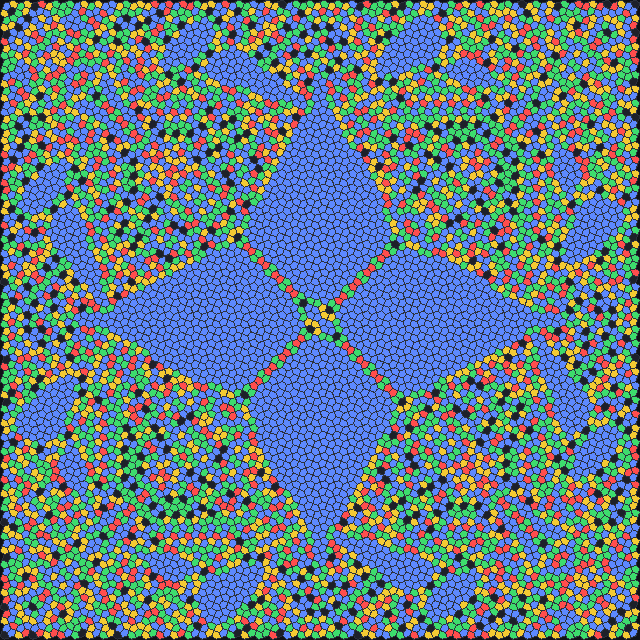
docs/scenes/automata/sandpile-identity-cairo.json.What it is
Each cell holds a whole number of grains. A cell with at least as many grains as it has neighbours is unstable: it topples, giving one grain to each neighbour and keeping the rest. Grains that would go past the edge of a finite grid are lost; the edge is a sink. Toppling continues until every cell is stable.
Two facts make the model special:
- Order does not matter. However the topplings are ordered, the final stable pile is the same. This is the abelian property that gives the model its name, and it means adding grains and then stabilising behaves like addition.
- The recurrent piles form a group. The stable piles that keep coming back when grains are added at random form a finite abelian group, the sandpile group. Every group has an identity element: here, the one recurrent pile that, added to any recurrent pile and stabilised, changes nothing. On a square grid this identity is an intricate fractal, and its shape depends on the shape of the grid.
A different classic experiment drops a great many grains on a single cell. The result is a large, roughly round pile with a fractal pattern inside that looks the same at every scale.
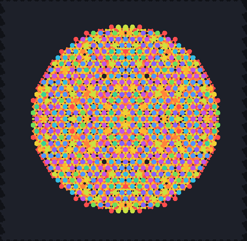
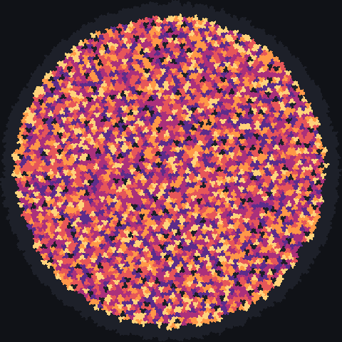
docs/scenes/automata/sandpile-pile-k2.json.
Right: 10,000 grains on the hat tiling, where tiles topple at 4, 5 or 6. Scene
docs/scenes/automata/sandpile-pile-hat.json.Where it came from
Per Bak, Chao Tang and Kurt Wiesenfeld proposed the sandpile in 1987 as an explanation of how systems can organise themselves into a critical state, in which avalanches of every size occur and their sizes follow a power law (Bak, Tang and Wiesenfeld 1987; 1988). Deepak Dhar showed in 1990 that the final state does not depend on the order of topplings, so that adding grains defines commuting operators and the recurrent configurations form an abelian group (Dhar 1990); Lionel Levine and James Propp credit the name “sandpile group” to Dhar (Levine and Propp 2010). Majumdar and Dhar later linked the model to spanning trees and the q → 0 Potts model (Majumdar and Dhar 1992).
The same dynamics have been invented several times under other names, including chip-firing; in combinatorics the main early reference is Björner, Lovász and Shor’s “Chip-firing games on graphs” (1991; see Levine and Propp 2010).
Michael Creutz drew attention to the identity element and its fractal structure on the square grid (Creutz 1991); Caracciolo, Paoletti and Sportiello call it the Creutz identity (Caracciolo, Paoletti and Sportiello 2008), and Le Borgne and Rossin studied it combinatorially (Le Borgne and Rossin 2002). Single-source piles on the square grid were studied by Srdjan Ostojic (Ostojic 2003), and Wesley Pegden and Charles Smart proved that the rescaled piles converge to a limit (Pegden and Smart 2013). Off the square grid, Fersula, Noûs and Perrot computed identities on triangular and hexagonal grids and on Penrose tilings (Fersula, Noûs and Perrot 2020).
How JETCARP runs it
The rule on any tiling
The rule is written Sandpile. A tile topples when its number of grains reaches its number of
neighbours, so the threshold is the tile’s degree in the neighbour graph: 4 on squares and 6 on
hexagons with edge neighbours, but anything from 3 to 12 on a 2-uniform tiling and 4 to 7 on the
spectre. Sandpiles use edge neighbours by default; with touch neighbours a square topples at 8. Dead
edges, and the open boundary of an aperiodic patch, are sinks. A wrapped grid has no sink, so it has
no identity and cannot absorb more grains than it can hold.
Starting piles include {"pile": {"grains": N}} (N grains on the centre tile) and random heights;
steps_per_gen sets how many toppling sweeps make one generation, so you can watch an avalanche
spread or let it settle quickly.
The identity
JETCARP computes the identity of the sandpile group as stab(2m − stab(2m)), where m is the pile in
which every tile holds one grain fewer than its threshold and stab means “topple until stable”. Its
tests check that the result is idempotent, stab(I + I) = I, on squares, hexagons, Cairo pentagons and
the spectre. The app’s Identity button and the scene command {"op": "sandpile", "action": "identity"} compute it on any tiling with sink edges.
Very large piles
jetcarp pile drops N grains on one tile of an unbounded grid. It never builds a tower of N grains:
it reads N’s binary digits from the most significant end and repeats s ← stab(2s + bit · δ), where δ is
one grain on the centre tile. The abelian property makes the result the same as stabilising all N
grains at once, while heights stay small at every step. The board grows as the pile does, so no grain
is ever lost, and on aperiodic tilings the pile is built on an exact patch of up to about 17 million
tiles. Piles can be toppled on the GPU on periodic tilings, and are saved after every doubling step so
a long run can be resumed. The app’s Sandpile… window builds one too, as a catalog job: it draws
the pile as it grows, and a stopped pile carries on from its last finished step, from the window, the
Hunts… window, or jetcarp jobs resume. See the guide Large sandpiles.
What is new here
Sandpile identities have been computed before on triangular, hexagonal and Penrose grids (see above), and on hexagonal and 4.8.8 grids in Eli T. Johnson’s master’s thesis (Johnson 2019); single-source piles on the square grid have a long literature. To our knowledge, JETCARP is the first to show sandpile identities and large single-source piles on the hat and spectre monotiles, on the k-uniform tilings with k of 2 or more, and on the Laves tilings other than the regular grids. The last are what the isohedral tilings amount to: a sandpile sees only the neighbour graph, and the 81 isohedral types have only the eleven graphs of the Laves tilings (see Isohedral tilings), so an identity on an isohedral type is an identity on its Laves tiling. Our search found no published sandpile work on the hat or spectre at all. The doubling method follows directly from the abelian property and is presumably known, so we do not claim it. The search is described in What is new in JETCARP.
Try it
- Quick Start: Abelian sandpile, Sandpile identity on Cairo pentagons, Sandpile on the Spectre, Sandpile on hexagons, and a sandpile on every tiling in the Tiling showcase.
jetcarp run docs/scenes/automata/sandpile-identity-cairo.json --png identity.pngjetcarp pile --tiling spectre --grains 1e6builds a million-grain pile on the spectre.
References
- Bak, Tang and Wiesenfeld 1987; Bak, Tang and Wiesenfeld 1988; Dhar 1990; Majumdar and Dhar 1992
- Björner, Lovász and Shor 1991; Levine and Propp 2010
- Creutz 1991; Le Borgne and Rossin 2002; Caracciolo, Paoletti and Sportiello 2008
- Ostojic 2003; Pegden and Smart 2013
- Fersula, Noûs and Perrot 2020
Von Neumann’s 29-state automaton
John von Neumann designed this automaton in the early 1950s to answer a question about life itself: can a machine build a copy of itself, including the instructions for building the next copy? Von Neumann’s answer was a universal constructor made of cells, each with 29 states, connected to its four neighbours. Conway’s Life began as a simplification of its ideas. JETCARP runs it on the square grid, from the rule as published.

docs/scenes/automata/vonneumann-channels.json.What it is
Every cell is in one of 29 states, and talks only to its four edge neighbours:
- Ground (unexcitable), the empty background.
- Transmission states: ordinary and special, each pointing in one of four directions, each quiescent or carrying a signal (16 states). A transmission cell passes a signal in the direction it points, one cell per step. A signal of the other kind (ordinary versus special) pointed at a transmission or confluent cell destroys it, turning it back to ground.
- Confluent states (4), which combine signals: a confluent cell fires only when all the ordinary cells pointing into it fire, and it delays its output, which lets it act as an AND gate and a memory element.
- Sensitised states (8), the intermediate steps by which a signal arriving at ground builds a new cell. A sequence of signals sent into ground decides, bit by bit, which of the other states the new cell becomes.
With these parts, a constructing arm can extend into empty space, build any pattern of cells by sending the right signal sequences, and withdraw again. Von Neumann’s design couples such an arm to a long tape of instructions; the machine reads the tape, builds a copy of itself, and copies the tape into it: self-reproduction from a description, a constructor and a copier.
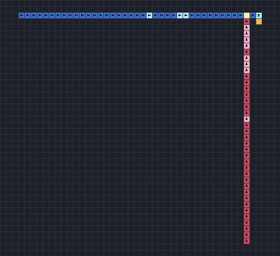
docs/scenes/automata/vonneumann-construct.json, 20 generations.Where it came from
Von Neumann’s work on automata began with “The General and Logical Theory of Automata” (1948) and a series of lectures at the University of Illinois in 1949, which described a kinematic self-reproducing machine built from mechanical parts. Arthur W. Burks writes that Stanisław Ulam suggested a cellular framework would be easier to treat mathematically. Von Neumann then designed an infinite array of square cells, each holding the same 29-state automaton. Von Neumann began the manuscript in September 1952 and worked on it until 1953, and left it unfinished (von Neumann 1966).
Burks edited and completed the work as Theory of Self-Reproducing Automata (1966), which states the transition rule and shows how to finish the self-reproducing design (von Neumann 1966). A footnote there notes that Edward F. Moore’s 1962 paper proposed the name “tessellation model” (Moore 1962). E. F. Codd later reduced the number of states to 8 (Codd 1968; see Rule tables).
The first working implementation of a self-reproducing universal constructor was built by Renato Nobili and Umberto Pesavento in 1994; to simplify the design they extended the rule so that confluent cells can cross signals (Pesavento 1995; Nobili and Pesavento 1996). Golly runs the original 29-state rule and the extended Nobili32 and Hutton32 variants (Golly: JvN), and Yinusa and Nehaniv used it to show that the completed machine passes heritable mutations to its offspring (Yinusa and Nehaniv 2011). Greg Turk’s 2025 review traces the line from von Neumann through Codd and Langton to the present (Turk 2025).
How JETCARP runs it
From the book
JETCARP’s JvN29 was written from Burks’s 1966 edition: the states and transition rule (section
2.8.1), its verbal summary (2.8.2) and the worked illustrations (2.8.3). The book’s formal statement
of the rule is garbled in the scanned text that was available, so the implementation follows the
clear verbal summary, which the legible parts of the formal rule agree with. Where the text left
details open, the choices were checked against the book’s own examples:
- A cell is destroyed by a signal of the other kind pointing at it from any side, including head on, so an ordinary and a special signal pointing at each other destroy each other.
- Destruction wins over receiving a signal but not over sending one: a cell excited at one step still delivers its signal at the next, even though it has become ground.
- In the storage loop of Fig. 12 the text says four cells store five bits, which four one-step cells cannot do, so one of them must be a confluent cell (a two-step delay). Starting it that way reproduces the book’s trace exactly.
- The construct-and-withdraw sequence of Fig. 14 builds its path, writes the confluent cell and withdraws in exactly the 37 ticks the book states.
The book is in copyright; only the rule, which is an algorithm, is reimplemented. No code, rule files or patterns from other programs were used. JETCARP numbers the states its own way (ground 0, sensitised 1 to 8, transmission 9 to 24, confluent 25 to 28), so its patterns are not interchangeable with other programs’ files.
Notation and display
The rule is written JvN29 (also JvN or VonNeumann29). The Draw tool lists the states by name.
Ordinary transmission cells are blue and special ones red, excited forms pale and bright; confluent
cells are green and sensitised ones amber. Pictures draw an arrow on each transmission cell when tiles
are at least 10 pixels across.
Square grid only
The rule depends on the four compass directions, so it has no meaning on other tilings, and JETCARP refuses to place it on one or to switch a world containing it to another tiling. Cells beyond a dead edge count as ground; wrapped edges work.
What is new here
Nothing. This is von Neumann’s automaton as Burks published it. JETCARP’s contribution is a fresh, documented reading of the book, with the ambiguities and how they were resolved written down.
Try it
- Quick Start: von Neumann: storage loops growing channels and von Neumann: construct and withdraw.
jetcarp run docs/scenes/automata/vonneumann-construct.json --gens 37 --png construct.pngruns the whole Fig. 14 sequence.
References
- von Neumann 1966; Moore 1962; Codd 1968
- Pesavento 1995; Nobili and Pesavento 1996; Golly: JvN; Yinusa and Nehaniv 2011; Turk 2025
Priority rules and the Spectre glider
For years it was an open question whether anything could glide across an aperiodic tiling: a small pattern that moves forever through a tiling that never repeats. In 2026 James Edmond found gliders on both of the new aperiodic monotiles, the hat and the spectre, by widening the space of rules to priority tables and searching it with an evolutionary algorithm. JETCARP runs Edmond’s rules, and reimplements that search on every tiling.

docs/scenes/automata/priority-spectre-glider.json, 64 generations.What it is
A priority table is a rule written as an ordered list of rows. Each row says: if the cell is in this state (or any state), and its neighbours meet these conditions, then its next state is this. The conditions are thresholds on how many neighbours are in each state, joined by “and”. The first row that matches decides the cell’s next state; a cell that matches no row becomes empty.
This is more expressive than a birth/survival rule, which only counts live neighbours, and it contains the Generations rules as a special case. Edmond found that searches over simpler rules on the hat and spectre turned up only travellers that eventually die, and that priority tables over the touch neighbourhood were rich enough to hold true gliders.
The Spectre glider rule is one such table with four states, of which it uses three. A head (state 1) excites wings (state 3) around it; a wing next to a head becomes a head; crowded wings die. The result is a relay that moves one ring of tiles every two generations. From the seed it emits two gliders on lanes 120° apart, and Edmond’s paper reports that its gliders travel a million rings at constant speed and heading (Edmond 2026).
Where it came from
Life on Penrose tilings was studied for its still lifes and oscillators; Hill, Stepney and Wan, and Owens and Stepney, found no moving objects (Hill, Stepney and Wan 2005; Owens and Stepney 2010). Adam P. Goucher found the first glider on an aperiodic tiling in 2012, with a four-state rule on a Penrose tiling (Goucher 2012); Edmond’s paper says this overturned a conjecture, backed by a small cash prize, that no such object exists. After the hat was announced in 2023, Andrew Trevorrow’s HatLife let people explore rules on it interactively, including a hand-designed “Worms” rule whose worms cross the patch (Trevorrow 2023).
James Edmond’s “Gliders on Aperiodic Monotilings: Cellular Automata on the Hat and Spectre” (2026) introduced priority tables, presented as Edmond’s own rule family, and found gliders on both monotiles with a genetic algorithm over four-state tables on the touch neighbourhood. The gliders’ headings fall on a “six-spoke compass”, and the Spectre glider is Edmond’s record of the evolved Spectre rule (Table 7 of the paper’s second version), found with no known rule planted in the search (Edmond 2026). Within weeks, Trevorrow’s HatLife and the new SpectreLife ran Edmond’s rules, SpectreLife with the glider rule modified to support eaters, oscillators and glider guns (Trevorrow 2026).
How JETCARP runs it
Notation
| Notation | Meaning |
|---|---|
SpectreGlider | Edmond’s Spectre glider rule |
Priority 4: 0|n0>=3&n1>=1->3; 3|n3>=3->0; 3|n1>=1->1 | The same rule written as a table |
Priority 4: 3|n2>=1->2; 0|n3>=2->0; 0|n2>=1->3; 0|n1>=1->2 | Edmond’s hat glider B in another table, as JETCARP’s search found it (below) |
Priority <states>: is followed by rows separated by semicolons. Each row is
<own state>|<conditions>-><next state>, where the own state is a number or * for any state, and the
conditions are terms nS>=m (“at least m neighbours in state S”) joined by &, or always. The
first matching row wins and the default is 0. SpectreGlider is exactly the three rows above: these
are the rows of Edmond’s Table 7 that do not lead to state 0, since 0 is the default anyway.
On any tiling
A priority table only counts neighbours by state, so it runs on any neighbour graph (see
How JETCARP generalises automata). Edmond’s rules use touch neighbours, which is
also JETCARP’s default for them. The seed glider_pair places the Spectre glider’s two-tile seed at
the centre of a patch.
Evolutionary search and verified movers
jetcarp search evolve reimplements Edmond’s evolutionary search and runs it on any tiling,
periodic or aperiodic. It is written from Edmond’s paper and a reading of Edmond’s repository; two small
functions, the mutation step and the table notation, are adapted from the monotile-ca code under its
MIT licence, as listed in JETCARP’s third-party notices. Movers it finds on aperiodic tilings are followed
across ever larger exact patches (jetcarp library movers track), or on a sliding window that
generates tiles around the mover as it goes (jetcarp search mover), and recorded as verified to
a distance: the number of rings of tiles the mover was followed without changing.

docs/scenes/automata/priority-hat-glider.json, 64 generations.What is new here
Priority tables, the evolutionary method, the Spectre glider and the hat gliders are Edmond’s. The hat glider JETCARP’s search found is Edmond’s hat glider B in another table: with B’s states renamed, the two tables agree on every configuration the glider meets, and run side by side they give the same states every generation (checked for 1,467 generations on a level-7 patch). JETCARP’s table has one extra row, and its seed launches the glider on a different lane, which is why it first looked like a different glider. Credit for it is Edmond’s.
JETCARP’s own part is running the search on every tiling and verifying movers to a distance. For this glider that meant following it on a sliding window for 1,000,000 rings of tiles, at a steady 2.14 units per generation; Edmond’s certificates already prove it immortal. We make no novelty claim for this family. The comparison is described in Findings.
Try it
- Quick Start: Spectre glider and Spectre glider (Edmond 2026).
jetcarp script docs/scenes/automata/glider-trail.rhai --out pictures --set scene=$PWD/docs/scenes/automata/priority-spectre-glider.json --set gens=70 --set png=trail.pngdraws the glider’s trail over 70 generations as one picture.jetcarp search evolve --helpdescribes the search. Each search is a catalog job, saved after every generation:jetcarp jobs resume JOBcarries on one that was stopped, ending exactly as an uninterrupted run would, and the app’s Hunts… window lists, stops, and resumes it. The app’s Catalog tools… window (the Evolve tab) starts one the same way, with Stop and Resume.
References
- Edmond 2026
- Goucher 2012; Hill, Stepney and Wan 2005; Owens and Stepney 2010
- Trevorrow 2023; Trevorrow 2026
Rule tables
Every family on the other pages has its rule built into JETCARP. A rule table is the way to write your own: a list of transitions, each saying “a cell in this state, with these neighbours in these positions, becomes this”. Rule tables can express almost any rule with a handful of states, including rules that depend on direction, which is how classic constructions such as Codd’s automaton and Langton’s loops are usually written down.

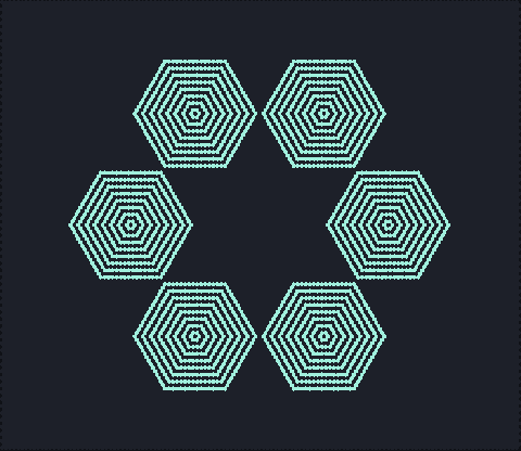
parity, in which each cell becomes the exclusive or of its
four edge neighbours, from one live cell for 63 generations. Watch the pattern copy itself: the rule is
linear, so at generation 2k the pattern is four copies of the starting cell, 2k
cells away, and each copy then replays the history so far; at generation 63, just before the next
doubling, the copies fill a diamond. Scene
docs/scenes/automata/ruletable-parity.json. Right: the same idea on hexagons, as a table
of 128 transitions written into the scene itself, 47 generations. Scene
docs/scenes/automata/ruletable-hex.json.What it is
A rule table lists transitions of the form c,n1,…,nk:new: if the cell is in state c and its
neighbours, read in a fixed order, are in states n1 to nk, its next state is new. Each position
can also be * (any state) or a set of alternatives such as 1|2|3. A symmetry setting saves
writing out every rotation of a case: rotate applies each transition to all rotations of the
neighbours, rotate_reflect also to their mirror images, and permute treats the neighbours as an
unordered collection. The first transition that matches wins; a cell that matches none keeps its
state.
Because a table can tell neighbours apart by position, it can express rules that depend on direction: a signal travelling along a wire, a gate that only lets it pass one way. That is what made tables the standard way to write constructions like Codd’s.
Where it came from
Edgar F. Codd’s PhD thesis at the University of Michigan (1965), advised by John H. Holland, and Codd’s book Cellular Automata (1968) reduced von Neumann’s 29 states to 8 while keeping computation and construction universal, with signals running along wires wrapped in a sheath (Codd 1965; Codd 1968; Wikipedia: Codd’s cellular automaton). Christopher Langton’s self-reproducing loop of 1984 was derived from Codd’s periodic emitter; it replicates with a few dozen cells but does not compute universally (Langton 1984). Rules like these are naturally written as transition tables. Tim Hutton found four flaws in Codd’s published specification, corrected them and built Codd’s complete self-replicating computer, whose tape alone is 208 million cells long (Hutton 2010).
Golly’s RuleTable format, written by Hutton, made tables a common exchange format (Golly: file formats; Golly credits), and Hutton’s Rule Table Repository collected Codd’s rule, John Devore’s 1973 variant, Langton’s loops and their successors by Byl, Chou and Reggia, and Sayama (Rule Table Repository).
How JETCARP runs it
JETCARP’s own format
JETCARP’s tables are its own JSON format; it does not read Golly’s files and uses none of Golly’s code. A table looks like this:
{
  "name": "parity-example",
  "states": 2,
  "neighborhood": "edge",
  "symmetry": "rotate",
  "arity": 4,
  "transitions": ["0,1,0,0,0:1", "1,1,1,0,0:0"]
}
arity is the number of neighbours each transition lists. A scene can carry its own tables in a
tables list, and the app can load one from a file; an automaton then uses it with the rule
Table <name>. One table is built in: Table parity, Fredkin’s replicator rule on edge neighbours
(each cell becomes the XOR of its four neighbours), generated in JETCARP from the rule’s definition.
Neighbour order on any tiling
The neighbours are read in the cell’s clockwise slot order, the same order turmites use for turning
(see How JETCARP generalises automata). On squares with edge neighbours that is
north, east, south, west. Edge neighbours are the default; touch neighbours can be chosen. Cells past a
dead edge read as 0 (or 1 with live edges). On a tiling where tiles have different numbers of
neighbours, a positional table only applies to tiles with exactly arity neighbours, and the others
keep their state; a permute table counts neighbours without regard to position.
Codd’s automaton
JETCARP v0.4.0 does not ship Codd’s rule; adding it, written from Codd’s book, is on the roadmap.
What is new here
Nothing. Rule tables are a standard tool; JETCARP’s contribution is only its own file format and running tables on any tiling’s neighbour order.
Try it
- Quick Start: Parity (von Neumann table).
jetcarp run docs/scenes/automata/ruletable-hex.json --gens 47 --png hex-parity.png, then edit the scene’s table and run it again.
References
- Codd 1965; Codd 1968; Wikipedia: Codd’s cellular automaton
- Langton 1984; Hutton 2010
- Golly: file formats; Golly credits; Rule Table Repository
Named rule catalogue
Generated page. Built by
docs/tools/gen-named-rules.pyfrom the program’s own rule list (crates/jetcarp-core/data/rules/named.json) and the credits filedocs/data/named-rule-credits.tsv. Edit those files, not this page.
JETCARP knows 166 rules by name, collected from the rule lists that the Life community
has kept for decades. You can type a name anywhere a rule is expected (jetcarp rules lists them, with
a few more built-in names for families that have no standard list). Every one of them runs on any
tiling, though most were found on the square grid and behave differently elsewhere; see
How JETCARP generalises automata.
About the credits. Most of these rules were named, and often found, by hobbyists: through Mirek Wójtowicz’s MCell program and its rules lexicon in the late 1990s, the ConwayLife.com forums, and LifeWiki’s lists. The Credit column names a person only when a source does, with the role the source gives (found, named, studied). An empty cell means no source we checked names anyone, not that nobody did. Where sources disagree, both are shown. 76 of the 166 rules have a named person. The credits were checked in November 2026 against LifeWiki (read through its mirror, since conwaylife.com refuses automated reading), the MCell lexicon, Toffoli and Margolus’s Cellular Automata Machines (1987) and Wikipedia. If you know of an earlier or missing credit, please open an issue.
The Source column links the list each rule was taken from. The short descriptions JETCARP shows for each rule are written in our own words.
| Family | Rules |
|---|---|
| Life-like | 88 |
| Life-like (B0) | 6 |
| Life-like, hexagonal | 1 |
| Life-like, von Neumann | 1 |
| Generations | 45 |
| Larger than Life | 9 |
| Elementary | 10 |
| Agents | 4 |
| Layered | 2 |
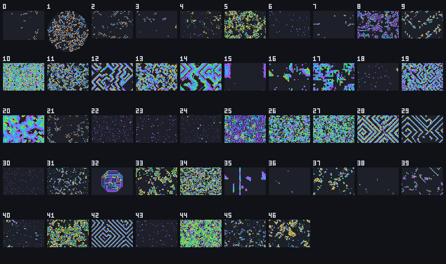
jetcarp quickstart --sheet --filter Generations. Numbers: 0 Brian's Brain; 1 Brian's Brain on Penrose rhombs; 2 Brian's Brain; 3 Star Wars; 4 Frogs; 5 Caterpillars; 6 Banners; 7 Transers; 8 Sticks; 9 Worms; 10 Lava; 11 Cooties; 12 RainZha; 13 BelZhab; 14 Xtasy; 15 Fireworks; 16 Bombers; 17 Faders; 18 9:43 at Knight; 19 BelZhab Sediment; 20 Bloomerang; 21 Brain 6; 22 Burst; 23 Burst II; 24 Chenille; 25 Circuit Genesis; 26 Ebb and Flow; 27 Ebb and Flow II; 28 Flaming Starbows; 29 Frozen Spirals; 30 Glisserati; 31 Glissergy; 32 Lines; 33 Living On The Edge; 34 Meteor Guns; 35 Nova; 36 OrthoGo; 37 Prairie on fire; 38 Rake; 39 SediMental; 40 Snake; 41 Soft Freeze; 42 Spirals; 43 Swirl; 44 Thrill Grill; 45 Transers II; 46 Wanderers.Life-like
Family page: Life-like.
Life-like (B0)
Family page: Life-like (B0).
| Name | Notation | Credit | Sources |
|---|---|---|---|
| AntiLife | B0123478/S01234678 | rule list; LifeWiki: List of Life-like rules | |
| InverseLife | B0123478/S34678 | Jason Rampe (named it; MCell: “a rule by”) | rule list; LifeWiki: List of Life-like rules; LifeWiki: OCA:B3678/S23; MCell lexicon |
| Invertamaze | B028/S0124 | rule list; LifeWiki: List of Life-like rules; LifeWiki: OCA:Invertamaze | |
| Neon Blobs | B08/S4 | rule list; LifeWiki: List of Life-like rules | |
| Oils | B014/S2 | rule list; LifeWiki: List of Life-like rules | |
| Wickstretcher And The Parasites | B01356/S012345 | rule list; LifeWiki: List of Life-like rules; LifeWiki: OCA:Wickstretcher And The Parasites |
Life-like, hexagonal
Family page: Life-like, hexagonal.
| Name | Notation | Credit | Sources |
|---|---|---|---|
| Hexagonal Life | B2/S34H | Name taken from the title of a ConwayLife.com forum thread by drc, 18 January 2016 (not re-checked) | rule list; LifeWiki: Hexagonal neighbourhood; ConwayLife forum |
Life-like, von Neumann
Family page: Life-like, von Neumann.
| Name | Notation | Credit | Sources |
|---|---|---|---|
| Gnarl (von Neumann) | B1/S0V | Kellie Evans | rule list; LifeWiki: Gnarl; MCell lexicon |
Generations
Family page: Generations.
Larger than Life
Family page: Larger than Life.
| Name | Notation | Credit | Sources |
|---|---|---|---|
| Bosco’s Rule | R5,C2,S33-57,B34-45 | Kellie Evans | rule list; LifeWiki: Larger than Life; MCell lexicon; Golly LtL help |
| Bugsmovie | R10,C2,S122-211,B123-170 | David Griffeath | rule list; LifeWiki: Larger than Life; MCell lexicon |
| Coexistence ¹ | R4,C2,S9,14,16-17,21,23-24,30-31,37-38,44-45,51-52,58-59,B3,10,17,21,24,31,38,45,52,59,NW100010001000000000000000000000777000100707001000777000000000000000000000100010001 | bubblegum | rule list; LifeWiki: Larger than Life |
| Factorio | R3,C2,S2,B3,N+ | H. H. P. M. P. Cole | rule list; LifeWiki: Larger than Life |
| Globe | R8,C2,S163-223,B74-252 | Mirek Wójtowicz | rule list; LifeWiki: Larger than Life; MCell lexicon |
| Majority (LtL) | R4,C2,S40-80,B41-81 | David Griffeath | rule list; LifeWiki: Larger than Life; MCell lexicon |
| Majorly | R7,C2,S112-224,B113-225 | David Griffeath | rule list; LifeWiki: Larger than Life; MCell lexicon |
| ModernArt | R10,C255,S1-2,B3 | Charles A. Rockafellor | rule list; LifeWiki: Larger than Life; MCell lexicon |
| Waffle | R7,C2,S99-199,B75-170 | Kellie Evans | rule list; LifeWiki: Larger than Life; MCell lexicon |
Elementary
Family page: Elementary.
| Name | Notation | Credit | Sources |
|---|---|---|---|
| Rule 105 | W105 | rule list; Wikipedia: Elementary cellular automaton | |
| Rule 126 | W126 | rule list; Wikipedia: Elementary cellular automaton | |
| Rule 150 | W150 | rule list; Wikipedia: Elementary cellular automaton | |
| Rule 18 | W18 | rule list; Wikipedia: Elementary cellular automaton | |
| Rule 184 | W184 | Earliest studies: Wentian Li (1987) and Krug & Spohn (1988); later used for traffic flow (e.g. Biham, Middleton & Levine 1992) | rule list; Wikipedia: Elementary cellular automaton; Wikipedia: Rule 184 |
| Rule 22 | W22 | rule list; Wikipedia: Elementary cellular automaton | |
| Rule 45 | W45 | rule list; Wikipedia: Elementary cellular automaton | |
| Rule 54 | W54 | rule list; Wikipedia: Elementary cellular automaton | |
| Rule 60 | W60 | rule list; Wikipedia: Elementary cellular automaton | |
| Rule 73 | W73 | rule list; Wikipedia: Elementary cellular automaton |
Agents
Family page: Agents.
| Name | Notation | Credit | Sources |
|---|---|---|---|
| Turmite LLRRRLRLRLLR | Turmite LLRRRLRLRLLR | rule list; Wikipedia: Langton%27s ant | |
| Turmite LRRRRRLLR | Turmite LRRRRRLLR | rule list; Wikipedia: Langton%27s ant | |
| Turmite RLR | Turmite RLR | rule list; Wikipedia: Langton%27s ant | |
| Turmite RRLLLRLLLRRR | Turmite RRLLLRLLLRRR | rule list; Wikipedia: Langton%27s ant |
Layered
Family page: Layered.
| Name | Notation | Credit | Sources |
|---|---|---|---|
| Layered parity | Layer 2/01 | Jimmie Rodgers (JETCARP, 2026) | JETCARP |
| Layered sum mod 3 | Layer 3/012 | Jimmie Rodgers (JETCARP, 2026) | JETCARP |
¹ Listed in the data file but not yet accepted by this version of JETCARP: Coexistence. Coexistence uses a weighted Larger than Life neighbourhood, which JETCARP does not read yet.
Tilings as neighbour graphs
A tiling covers the plane with tiles, leaving no gaps and no overlaps. For a cellular automaton, what matters about a tiling is not the shapes of its tiles but who is next to whom: its neighbour graph. JETCARP builds that graph for every tiling it supports, and every rule runs on the graph. This page explains how the graph is made and why two very different-looking tilings can be the same thing as far as an automaton is concerned.
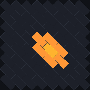
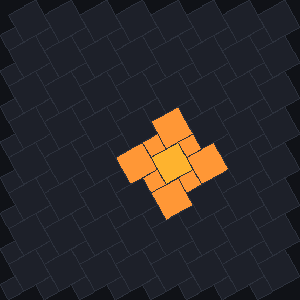
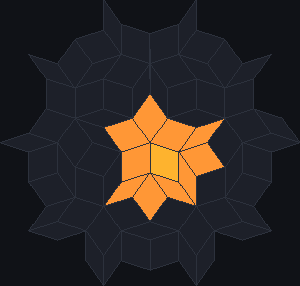
docs/scenes/tilings/graph-brick.json, graph-pyth.json and
graph-rhomb.json, 1 generation of a rule that switches on every cell with exactly one live
neighbour.What it is
The neighbour graph has one node for each tile and a link between every two tiles that are neighbours. There are two kinds of neighbour (see How JETCARP generalises automata):
- Touch neighbours share any part of their boundary: an edge or just a corner.
- Edge neighbours share a stretch of edge, not just a point.
A tile’s number of neighbours is its degree. In a tiling with one kind of tile placed the same way everywhere, every tile has the same degree; in mixed tilings the degree depends on the tile; in aperiodic tilings it varies irregularly across the plane. The tiling catalogue lists the degrees of every tiling.
Many tilings that look different have the same graph. A brick wall in running bond has the same neighbour graph as the hexagon tiling, and so does a herringbone pattern: each tile meets six others in the same arrangement. Escher’s lizards, on the three-fold hexagon tile, are hexagons as far as a rule is concerned. Any rule that only counts neighbours behaves identically on tilings whose graphs are the same, so a pattern found on one is a pattern on the other. This matters for honest claims. Every isohedral tiling has the graph of one of the eleven Laves tilings, so JETCARP’s 81 isohedral types are only eleven worlds for a rule: 30 of them are the square grid, 19 the hexagonal grid, 8 the triangular grid and 3 the Cairo tiling (see Isohedral tilings). Spaceships first found on isohedral tilings were Conway’s glider and its relatives in a different drawing. Likewise the quadrilateral, glide and four-fold families are squares and the Pythagorean tiling is 4.8.8. JETCARP compared all 362 combinations of its tiling families, isohedral types and 2- and 3-uniform tilings with both neighbourhoods and found 196 distinct graphs (Findings).
Rules that turn, such as Langton’s ant, also need the order of a tile’s neighbours around it, so JETCARP keeps each tile’s neighbours in clockwise order. And one family, Lenia, uses actual distances between tile centres, so for it the geometry matters too.
Where it came from
The standard reference on tilings is Branko Grünbaum and G. C. Shephard’s Tilings and Patterns, which defines the terms used here, such as edge-to-edge tilings and the symmetry groups of periodic tilings (Grünbaum and Shephard 1987; 2nd edition 2016). Treating the cells of an automaton as the nodes of a graph is a standard idea; the earliest automata already defined their neighbourhoods as fixed sets of nearby cells, named after John von Neumann and Edward F. Moore (Moore 1962). General tools that run rules on arbitrary polygon meshes, such as Ready, work the same way (Ready).
How JETCARP runs it
Building the graph
JETCARP stores a tiling in one of three ways, depending on its kind:
| Storage | Used for | How neighbours are found |
|---|---|---|
| Dense | lattices of one tile (squares, hexagons, bricks, any quadrilateral) | a fixed stencil of offsets |
| Periodic | a unit cell of several tiles repeated (Archimedean, k-uniform, isohedral, Cairo, herringbone, Pythagorean, drawn tiles) | a table of offsets for each tile in the cell |
| Explicit | finite patches of aperiodic tilings (Penrose, hat, spectre) | each tile’s neighbour list, written out |
For tilings that are not edge to edge, such as herringbone, the Pythagorean tiling and tiles you draw yourself, JETCARP measures contact from the geometry: two tiles are edge neighbours if they share a stretch of boundary and touch neighbours if they share any point. The tests check tilings for overlaps and gaps.
Size and edges
A periodic world is a rectangle of whole unit cells, given either as a number of cells (roughly square) or as a width and height in unit cells. Its edges can be dead (cells beyond count as empty), wrapped (a torus, so the tiling has no edges at all) or live (cells beyond count as alive). An aperiodic world is a patch of a chosen level, from 10 tiles at level 1 to about 35,000 at level 5 and about 18 million at level 8, always the tiles nearest a fixed centre, so smaller patches sit inside larger ones. Aperiodic patches have dead edges.
Different tilings, same rule
Because rules only see the graph, any scene can switch tiling and keep its rules (apart from the few
families tied to one grid; see How JETCARP generalises automata).
jetcarp tilings and jetcarp isohedral print the degrees JETCARP measures.
What is new here
Nothing on this page is new as an idea. What JETCARP adds is breadth: the same graph model for the regular, Archimedean, k-uniform, isohedral, drawn and aperiodic tilings, so that every rule runs on all of them. JETCARP’s exploratory search also treats the tiling itself as one of the dimensions it explores; see What is new in JETCARP.
Try it
jetcarp tilingslists every tiling family with its edge and touch degrees.- Run the same rule on the brick tiling and on hexagons: it behaves the same way on both, because the graphs are the same.
jetcarp run docs/scenes/tilings/graph-rhomb.json --gens 1 --png rhomb.png
References
Regular and Archimedean tilings
The regular tilings, by triangles, squares or hexagons alone, are the grids most cellular automata were born on. Add the eight Archimedean tilings, which mix regular polygons so that every corner looks the same, and you have the eleven uniform tilings of the plane. Each gives a rule a different neighbour graph: some tiles see three neighbours, some eighteen, and in the mixed tilings neighbouring tiles see different numbers. JETCARP runs every rule on all eleven.
triangle
square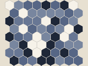
hex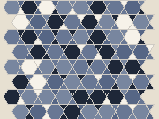
trihex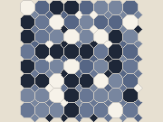
oct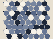
trunchex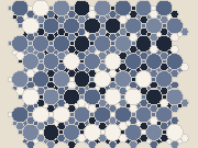
trunctrihex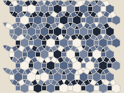
rhombitrihex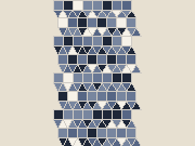
elongtri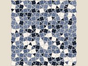
snubsq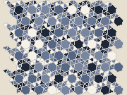
snubhexThe eleven uniform tilings, named by their vertex configurations, with JETCARP's family ids. Thumbnails from the tiling catalogue, drawn by JETCARP with each tile in a random colour.
What it is
A tiling by regular polygons is edge to edge when tiles meet only along whole edges, corner to corner. It is uniform (or 1-uniform, Archimedean) when every vertex looks the same: the same polygons, in the same order, meet at each corner. A vertex is described by listing the polygons around it, so 4.8.8 means a square and two octagons, and 3.3.4.3.4 means triangle, triangle, square, triangle, square. Repeated numbers can be written with exponents: 36 for six triangles, 32.4.3.4 for the snub square.
There are exactly eleven: the three regular tilings 36, 44 and 63, and the eight mixed ones 3.6.3.6 (trihexagonal, also called kagome), 4.8.8 (truncated square), 3.12.12 (truncated hexagonal), 4.6.12 (truncated trihexagonal), 3.4.6.4 (rhombitrihexagonal), 3.3.3.4.4 (elongated triangular), 3.3.4.3.4 (snub square) and 3.3.3.3.6 (snub hexagonal), which comes in two mirror-image forms.
For an automaton the differences are large. With touch neighbours a triangle in the triangular tiling has 12 neighbours, a hexagon 6; in 3.3.3.3.6 each hexagon touches 18 tiles and each triangle 9. In 3.12.12, touch and edge neighbours are the same (3 for a triangle, 12 for a dodecagon), because no two tiles meet at a corner only. Rules that count neighbours respond to all of this.

B4,5,7,8,10,11/S0,2,3,4,6,7,9,10, one generation per frame. Hexagons here touch 12 tiles and
triangles 6, which is why the rule lists counts up to 11; watch the activity run back and forth along
the row of hexagons. Found by JETCARP's soup search. Scene
docs/scenes/tilings/osc-trihex-p42.json.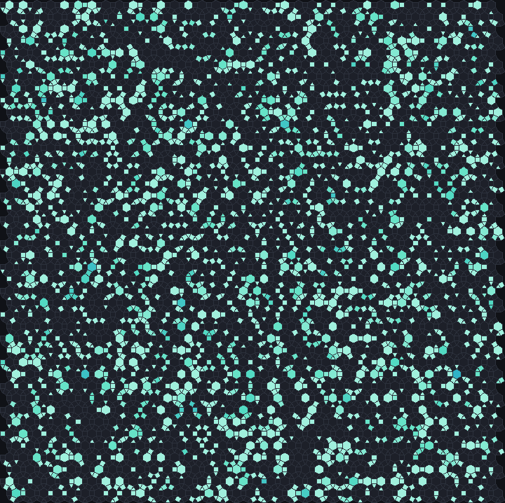
docs/scenes/tilings/archimedean-rhombitrihex.json.Where it came from
The regular tilings are ancient as patterns. The first systematic mathematical treatment of edge-to-edge tilings by regular polygons, including the eight further Archimedean tilings, is Johannes Kepler’s in Book II of Harmonices Mundi (1619) (Kepler 1619; English translation Kepler 1997). Darrah Chavey’s 1984 thesis examined Kepler’s results in detail (Chavey 1984). Branko Grünbaum and G. C. Shephard surveyed the subject “from Kepler to the present” in 1977 and in their book Tilings and Patterns, the standard modern reference (Grünbaum and Shephard 1977; 1987).
The dotted vertex notation (4.8.8) is commonly named after H. M. Cundy and A. P. Rollett’s Mathematical Models (Cundy and Rollett 1961); Grünbaum and Shephard use exponents. Later notations designed for generating tilings automatically include the GomJau-Hogg notation (Gomez-Jauregui et al. 2021).
Cellular automata on these tilings have their own history. Carter Bays studied Life-like rules on the triangular tiling (Bays 1994) and on hexagons and Cairo pentagons (Bays 2005), and wrote an overview (Bays 2009). In June 2013 EricG emulated all eight mixed Archimedean tilings and their duals in Golly, with cells that share an edge or a vertex as neighbours, and reported spaceships in Life-like rules on every one of the eight, in Life itself on 3.6.3.6, 3.3.4.3.4 and 3.3.3.4.4 (EricG 2013); EricG named rules but did not list the ships, and the pattern files are no longer online. A 2014 Code Golf challenge ran Life on several non-square tilings; Peter Taylor found only oscillators on 3.4.6.4 (Code Golf 2014). H. S. Guttesen ran Life on six of the mixed Archimedean tilings, described gliders on 3.6.3.6 and 3.3.4.3.4 and built a glider gun on 3.6.3.6 (Guttesen 2026).


B3/S23). Left: glider g on the kagome tiling
3.6.3.6, two hexagons and a trailing triangle, period 4, one lattice step every four generations.
Right: the period-8 glider on the snub square tiling 3.3.4.3.4, a ring of triangles with one square,
moving two lattice steps every eight generations. JETCARP's soup searches found both independently;
watch how each tile kind takes its turn. Scenes
docs/scenes/tilings/glider-guttesen-kagome.json and
glider-guttesen-snubsq.json.How JETCARP runs it
The triangle, square and hexagon tilings are reshapeable families (triangle, square, hex):
their tiles can be any triangle, any parallelogram or any of a family of hexagons, and the regular
shapes are the default (see Editable tile families). The eight mixed tilings are
fixed families: trihex, oct, trunchex, trunctrihex, rhombitrihex, elongtri,
snubsq and snubhex. All eleven also appear in the k-uniform catalogue as its
k = 1 entries, k1-001 to k1-011.
In a scene the tiling is given by its family id, a size and an edge rule, for example
"tiling": {"family": "rhombitrihex", "size": {"cells": 9000}, "boundary": "wrap"}. A flat-topped
version of the hexagon tiling, hex_flat, exists for the three-parent
hexagonal row rules.
What is new here
The tilings are classical. On them, JETCARP’s searches have found spaceships in Life-like rules on
4.8.8, 3.12.12, 4.6.12, 3.4.6.4, 3.3.3.4.4 and 3.3.3.3.6, and on 3.6.3.6 in rules other than Life. After
the checks described in What is new in JETCARP, six
single ships with no flag remain on these tilings, four on 3.3.3.4.4 and one each on 3.4.6.4 and
3.3.3.3.6. They run in none of the rules in which EricG reported ships, and to our knowledge they have
not been reported before. Three of the four on 3.3.3.4.4 were found in strips of squares and triangles
inside 2- and 3-uniform tilings; their live tiles evolve the same way on the elongated triangular tiling
itself, so they are listed there. Two ships on 4.8.8 and two on 3.12.12 passed the same checks but run in
the B2 and B26 rules where EricG saw many ships, so they are flagged until EricG’s patterns can be
compared. Four ships are below.
The others on these tilings are described rather than claimed. On 4.8.8, 3.12.12, 4.6.12, 3.6.3.6 and
3.3.3.4.4 the rest are small ships that turn up often in soups, ships in well-known rules such as HighLife or
B2/S34, or a smaller ship with a passenger, and others may well have seen them. Guttesen’s Life
gliders on 3.6.3.6 and 3.3.4.3.4 (on tilings where EricG had seen Life spaceships in 2013), which
JETCARP also found, are Guttesen’s, and so are the pairs of them that
JETCARP’s catalogue first listed as separate ships. In Life on 3.3.4.3.4, JETCARP also found two larger
ships built around Guttesen’s glider, of periods 16 and 24; we found no earlier report of them. Every ship is
listed in Findings.
A census of Life itself, 50,000 random soups on each of the eleven tilings, found spaceships only on the square grid, 3.6.3.6, 3.3.4.3.4 and 3.3.3.4.4 (see Life on the Archimedean and k-uniform tilings). On the first three they are Conway’s and Guttesen’s ships, the pairs and bound pairs those form, and the larger snub-square ships above. On 3.3.3.4.4 it is one ship, now and then flying in a pair: eight to twelve cells, period 2, moving along the rows at c/2, in about one soup in eleven. It is probably the “common spaceship (although it only travels horizontally)” that EricG reported there in 2013, although EricG’s patterns are not online to compare. On the hexagonal and triangular grids, 4.8.8, 3.12.12, 4.6.12, 3.4.6.4 and 3.3.3.3.6 no soup produced a Life ship; on the last five, Guttesen and the 2014 Code Golf challenge had found none either.


57a0326c on 3.4.6.4, period 42, moving 3 lattice steps per period, in
the 1,024 rules from B3/S235 up. Right: d3cd3951 on 3.3.3.3.6, period 27, one
lattice step along a row per period, in about a million rules from B37/S2,5,6,10 up. Watch
each ship pass through shapes that look nothing alike before it repeats one place further on. Scenes
docs/scenes/tilings/ship-57a0326c.json and ship-d3cd3951.json.

3e30b9ff on 3.3.3.4.4, period 8, two lattice steps along the rows per
period, in the 1,024 rules from B46/S3458 up. Right: 504fdf46 on 4.8.8,
period 6, two lattice steps per period, in the 128 rules from B2/S2 up; it is one of the
flagged 4.8.8 ships, since EricG found many ships in B2 rules there. Scenes
docs/scenes/tilings/ship-3e30b9ff.json and ship-504fdf46.json.Try it
- Quick Start, family Tiling showcase: a lively rule and a sandpile on each of the eleven.
jetcarp run docs/scenes/tilings/archimedean-rhombitrihex.json --gens 200 --png 3464.png- Run Life (
B3/S23) ontrihexfrom a random start and look for small gliders, as Guttesen did. jetcarp run docs/scenes/tilings/ship-57a0326c.json --gens 126 --png ship.pngruns the period-42 ship for three periods.
References
- Kepler 1619; Kepler 1997; Chavey 1984
- Grünbaum and Shephard 1977; Grünbaum and Shephard 1987
- Cundy and Rollett 1961; Gomez-Jauregui et al. 2021
- Bays 1994; Bays 2005; Bays 2009; EricG 2013; Code Golf 2014; Guttesen 2026
k-uniform tilings
Allow more than one kind of corner and the eleven uniform tilings grow into an enormous family. A tiling by regular polygons is k-uniform when its corners fall into k classes: within a class every corner is the same, but the classes differ. JETCARP carries Brian Galebach’s complete catalogue up to k = 6, all 1,248 tilings, and every rule runs on each of them.
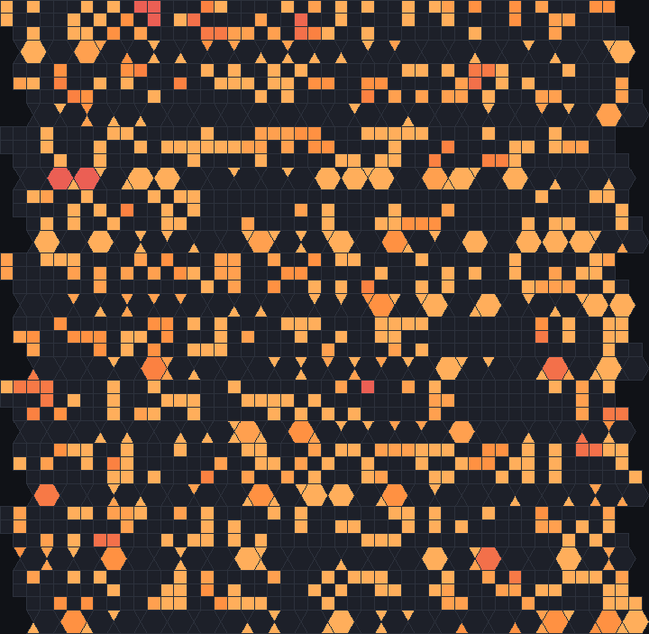
k3-011), 100 generations after a random start. Scene
docs/scenes/tilings/kuniform-k3-011.json.What it is
In an edge-to-edge tiling by regular polygons, two corners are equivalent if a symmetry of the whole tiling (a translation, rotation or reflection that maps the tiling onto itself) carries one onto the other. The tiling is k-uniform if there are exactly k classes of corner. The 1-uniform tilings are the eleven Archimedean tilings. With k = 2 there are 20, and the numbers grow quickly:
| k | Tilings in JETCARP’s catalogue | Catalogue ids |
|---|---|---|
| 1 | 11 | k1-001 to k1-011 |
| 2 | 20 | k2-001 to k2-020 |
| 3 | 61 | k3-001 to k3-061 |
| 4 | 151 | k4-001 to k4-151 |
| 5 | 332 | k5-001 to k5-332 |
| 6 | 673 | k6-001 to k6-673 |
A tiling’s name lists the vertex type of each class, in square brackets: [3.4.6.4; 4.6.12] has one
class of corners where a triangle, two squares and a hexagon meet and another where a square, a
hexagon and a dodecagon meet. When different tilings share a name, a number is added (#1, #2).
Mixing polygons this way gives tilings where neighbouring tiles have very different degrees, which
changes how rules behave from one region to the next.
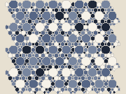
k2-001[3.4.6.4; 4.6.12]
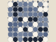
k2-002[3.4.3.12; 3.12^2]
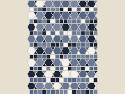
k2-007[3.4^2.6; 3.6.3.6] #2
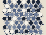
k2-013[3^6; 3^2.4.12]
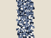
k3-011[3.4^2.6; 3.6.3.6; 4^4] #1
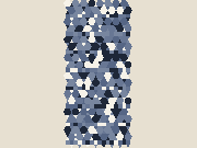
k3-030[3.4^2.6; 3.6.3.6; 3.6.3.6] #1
Six of the 2- and 3-uniform tilings. The full list, with neighbour counts, is in the tiling catalogue.
Where it came from
Otto Krötenheerdt classified the k-uniform tilings in which every class has a different vertex type in three papers in 1969 and 1970 (Krötenheerdt 1969; 1970; 1970b). Branko Grünbaum and G. C. Shephard treated k-uniform tilings in their 1977 survey and in Tilings and Patterns (Grünbaum and Shephard 1977; 1987). Darrah Chavey’s 1984 thesis gave the number of 3-uniform tilings, 61, and Chavey’s 1989 paper is the standard printed catalogue (Chavey 1984; Chavey 1989).
Brian Galebach wrote a program that generates complete sets of k-uniform tilings. Galebach’s entry in the On-Line Encyclopedia of Integer Sequences records 151 4-uniform and 332 5-uniform tilings (2002) and 673 6-uniform tilings (2003); Galebach’s page says the 6-uniform run took about a month of computation and reproduced Krötenheerdt’s list (Galebach, OEIS A068599; Galebach, n-uniform tilings). Marek Čtrnáct later extended the counts to k = 13 and, with Eryk Kopczyński, built an online tessellation catalogue (Čtrnáct and Kopczyński).
José Ezequiel Soto Sánchez, Tim Weyrich, Asla Medeiros e Sá and Luiz Henrique de Figueiredo gave an integer representation for periodic tilings by regular polygons (Soto Sánchez et al. 2021; see also Medeiros e Sá et al. 2018), and Soto Sánchez publishes Galebach’s collection in that form, with an online viewer, under the CC BY 4.0 licence (Soto Sánchez, tiling viewer). That file is JETCARP’s source.
How JETCARP runs it
JETCARP includes Soto Sánchez’s Galebach file unchanged, with attribution under its CC BY 4.0 licence. A
script rebuilds each tiling exactly, in coordinates that are whole-number combinations of twelfth roots
of unity, finds its translation lattice, symmetry group and vertex classes, and rejects anything
inconsistent. The tilings are numbered kN-NNN in Galebach’s order. (The one exception to exact
coordinates is 4.8.8, whose octagons need different numbers; it is built separately.)
In a scene a catalogue tiling is a periodic tiling with a catalogue id:
"tiling": {"family": "periodic", "params": {"catalog": "k3-011"}, "size": {"cells": 9000}}. Scripts
accept the id directly as the tiling (world(#{ tiling: "k3-011" })). In the app, the tiling panel’s
Tiling catalog lists every tiling and can be filtered by k or searched by vertex type or symmetry
group.
What is new here
The catalogue is Galebach’s, and the data and its representation are Soto Sánchez and colleagues’. What JETCARP adds is running cellular automata on all of it. Our prior-art search found no published cellular automaton work on k-uniform tilings with k of 2 or more. JETCARP has computed sandpile identities and piles across the catalogue, and its searches have found Life-like spaceships on 2- and 3-uniform tilings. No 2- or 3-uniform tiling has the neighbour graph of a lattice, of Cairo or of an Archimedean tiling (the k-uniform tilings with k from 4 to 6 have not been surveyed), so a ship found on one is not a lattice ship in disguise.
A k-uniform tiling can still contain a corridor of a simpler tiling, and a ship that runs in such a corridor belongs to the simpler tiling. JETCARP’s skeptical pass checked every ship against all the 2- and 3-uniform tilings: eight ships found on 3-uniform tilings run unchanged on a 2-uniform tiling or on 3.6.3.6, and are claimed there, and others run on several tilings of the same k. A looser congruence test, which asks only that the live tiles evolve the same way whatever the neighbour counts of the empty tiles around them, moved eight more: five ships of strips of squares and triangles run on the Archimedean tiling 3.3.3.4.4, and three 3-uniform ships run on a 2-uniform tiling. It also showed that two pairs of catalogue entries are one ship each. After those checks, 13 single ships with no flag on 2-uniform tilings and 6 on 3-uniform tilings are, to our knowledge, new; a few more are flagged because they were very common in their search or run in HighLife. All are listed in Findings; see also What is new in JETCARP.
Those ships run in rules other than Life. A census of Life itself (B3/S23), 50,000 random soups on
each of the 81 2- and 3-uniform tilings, found Life spaceships on 5 of the 20 2-uniform tilings and on
19 of the 61 3-uniform ones. To our knowledge, Life had not been reported on any 3-uniform tiling
before, nor on any 2-uniform tiling but k2-007, where Martin Büttner very likely found a period-20 ship
in 2014; other rules had been run on k2-001, [3.4.6.4; 4.6.12], without ships (see
What is new in JETCARP). Most of what the census found is common ships flying in pairs, or ships of simpler tilings
running in corridors; the single ships that passed every check are in
Life on the Archimedean and k-uniform tilings.

B45/S34 up. The same ship runs unchanged on k2-004
and in corridors of the 3-uniform tilings k3-010 and k3-016, where the search first found it. Its live
tiles also evolve the same way on k3-013, k3-019, k3-051, k3-052 and on the Archimedean tiling 3.3.3.4.4,
where the tiles beside its strip have more neighbours, so it is listed on 3.3.3.4.4, and flagged there as
small and common. Watch the triangles at its front and back take turns. Scene
docs/scenes/tilings/ship-d8692b4b.json.Treating the tiling as a dimension of an exploratory search also depends on having this catalogue.
Try it
- Quick Start, family Tiling showcase: entries on
k2-001,k2-002,k3-011,k4-100,k5-058andk6-673. jetcarp run docs/scenes/tilings/kuniform-k3-011.json --gens 200 --png k3-011.png- In a script,
for id in catalog_tilings(2) { ... }loops over the 2-uniform tilings.
References
- Krötenheerdt 1969; Krötenheerdt 1970; Krötenheerdt 1970b
- Grünbaum and Shephard 1977; Grünbaum and Shephard 1987; Chavey 1984; Chavey 1989
- Galebach, OEIS A068599; Galebach, OEIS A068600; Galebach, n-uniform tilings; Čtrnáct and Kopczyński
- Soto Sánchez et al. 2021; Medeiros e Sá et al. 2018; Soto Sánchez, tiling viewer
Isohedral tilings
An isohedral tiling uses a single tile shape, placed so that every tile is surrounded in exactly the same way: some symmetry of the tiling carries any tile onto any other. Escher’s drawings of birds, fish and lizards interlocking across the page are, almost all, isohedral tilings with decorated tiles. There are 93 types, and JETCARP supports the 81 of them that can be told apart by the tile’s shape alone, each with sliders that reshape the tile within its type.
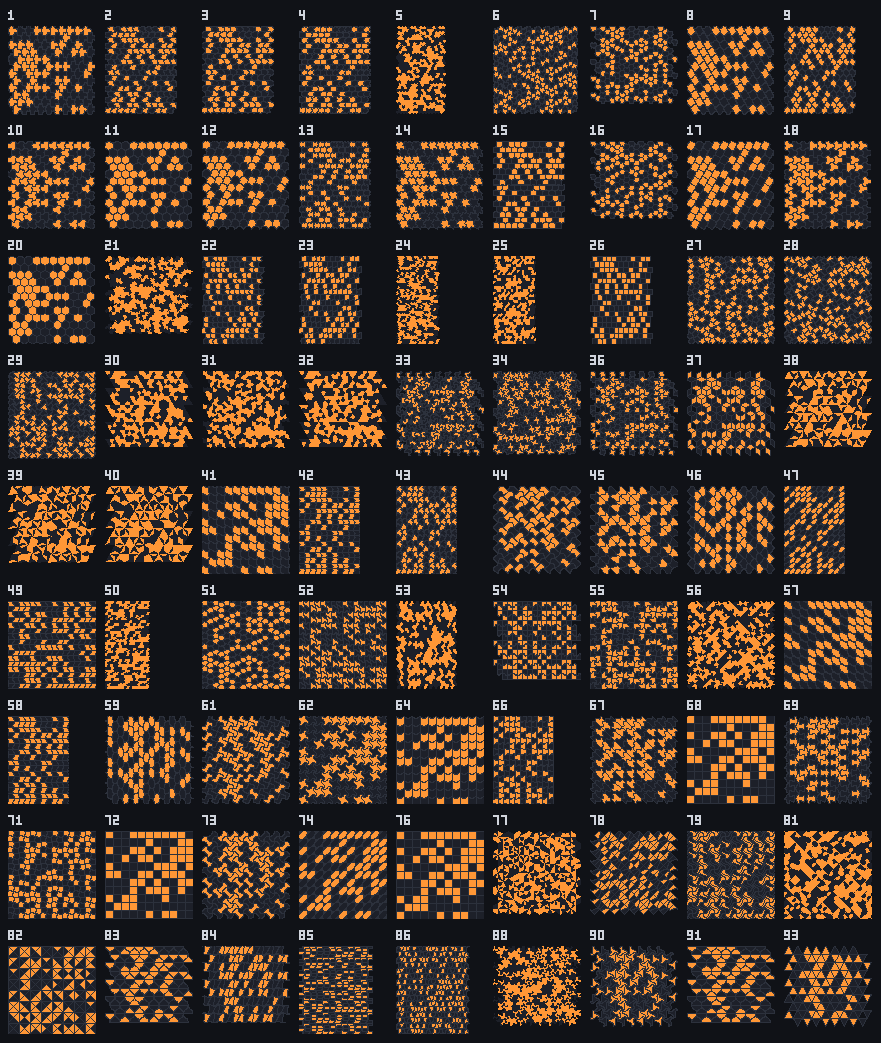
jetcarp isohedral --png sheet.png --cols 9 --thumb 88.What it is
Grünbaum and Shephard sorted isohedral tilings into 93 types, IH1 to IH93, by the way each tile’s edges and corners relate to its neighbours’: which edges must match which, and by what symmetry (a slide, a half turn about the edge’s midpoint, a rotation about a corner, a reflection). Within a type, a tile can change shape freely as long as those relations hold. Twelve of the types are marked: they need a motif drawn inside the tile to cut its symmetry down, so as bare shapes they coincide with other types. That leaves 81 types that can be told apart by shape alone.
For an automaton, the type fixes the neighbour graph, whatever the parameters: reshaping a tile changes the picture but not which tiles touch. Many types give the hexagonal graph (six neighbours each); others give the square grid’s or something else. The same rule can behave very differently on two tilings that look alike, and identically on two that look different; the tiling catalogue lists each type’s degrees, and the next sections show that there are only eleven graphs in all.
docs/scenes/tilings/isohedral-ih28.json.Where it came from
Elli and Heinrich Heesch completed a classification of 28 types of asymmetric tiles that give isohedral tilings in 1932; they submitted it in 1934 but chose not to publish, and tried for years to patent it (Reichenberger 2023). Heesch and Otto Kienzle published the 28 types in Flächenschluß (1963), with each tile’s boundary described as a word in letters for its edge symmetries; their scheme leaves out tilings with mirror lines (Heesch and Kienzle 1963; Kaplan and Schattschneider 2025).
Branko Grünbaum and G. C. Shephard gave the complete classification, with “incidence symbols”, in “The eighty-one types of isohedral tilings in the plane” (1977) and a polygonal version in 1978: 93 types, of which twelve are marked (Grünbaum and Shephard 1977; 1978; 1987). Nearly all of M. C. Escher’s regular divisions of the plane can be read as isohedral tilings (Kaplan and Schattschneider 2025); Doris Schattschneider’s Visions of Symmetry is the standard catalogue of Escher’s periodic drawings (Schattschneider 1990). Tom McLean’s online catalogue gives a template for each of the 93 types (McLean).
Craig S. Kaplan brought the types into computer graphics. Kaplan’s thesis and work with David Salesin on “Escherization” derive Escher-like tilings from shapes a user supplies (Kaplan 2002; Kaplan and Salesin 2000), and Kaplan’s book explains the types for programmers (Kaplan 2009). Kaplan’s Tactile library, in C++ and JavaScript, represents all 81 non-trivial types and lets their tiles be reshaped (Tactile; TactileJS).
How JETCARP runs it
JETCARP’s isohedral families ih01 to ih93 (81 of them) are converted from TactileJS’s tables, used
under Kaplan’s BSD 3-Clause licence. Each type has Tactile’s parameters (from none to six) and its edge
shapes: free curves, curves mirrored about their midpoint, half-turn symmetric curves, and straight
lines. Tactile’s description of each type gives the unit cell, so the usual periodic storage,
wrapped or dead edges, drawing and automata all apply. In a scene:
"tiling": {"family": "ih28", "params": {"p": [0.45, 0.5]}}; without p, Tactile’s default shape
is used.
In the app, pick Isohedral IH01–IH93 in the family list, then the type and its parameter sliders;
Edit tile… lets you drag corners and reshape edges, and the editor keeps the tile within its type.
jetcarp isohedral lists the types with their symmetry groups and neighbour counts, and
jetcarp isohedral --png sheet.png draws them all, as above.
Eleven graphs: the Laves tilings
Every isohedral tiling is combinatorially one of the eleven Laves tilings, the duals of the eleven uniform tilings: count the tiles meeting at each corner of a tile, and the sequence (written in brackets, such as [32.4.3.4] for the Cairo tiling) is one of eleven (Grünbaum and Shephard 1987). An isohedral tiling and its Laves tiling are the same tiling topologically, with the same edge and touch neighbour graphs, so a rule that only counts neighbours behaves on the one exactly as on the other. JETCARP’s survey of neighbour graphs sorted the 81 types as follows (Findings):
| Laves tiling | Types | A rule sees |
|---|---|---|
| [36] | IH01–IH18, IH20 | the hexagonal grid |
| [44] | 30 types from IH41 to IH76 | the square grid |
| [63] | IH83–IH86, IH88, IH90, IH91, IH93 | the triangular grid |
| [32.4.3.4] | IH27–IH29 | the Cairo tiling |
| [33.42] | IH22–IH26 | the prismatic pentagonal tiling |
| [34.6] | IH21 | the floret pentagonal tiling |
| [3.6.3.6] | IH33, IH34, IH36, IH37 | the rhombille tiling |
| [3.4.6.4] | IH30–IH32 | the deltoidal trihexagonal tiling |
| [3.122] | IH38–IH40 | the triakis triangular tiling |
| [4.82] | IH78, IH79, IH81, IH82 | the tetrakis square tiling |
| [4.6.12] | IH77 | the kisrhombille tiling |
So 57 of the 81 types are the three regular grids in another drawing and three more are the Cairo tiling. The shapes still matter for pictures, and for Lenia, which measures distances between tile centres; for every other rule family the eleven rows above are all there is.
What is new here
The classification is Grünbaum and Shephard’s and the tables are Kaplan’s. Cellular automata on a few isohedral tilings are not new either: Matej Kerekrety ran Life-like rules on the rhombille and Cairo tilings (Kerekrety 2020). JETCARP runs every rule on all 81 types and lets their tiles be reshaped while a rule runs.
For the rules, though, 81 types are not 81 worlds. As the section above explains, they have only the eleven neighbour graphs of the Laves tilings, so we present every result on an isohedral type as a result on its Laves tiling. Sandpile identities on the Laves tilings other than the square, hexagonal and triangular grids have not, to our knowledge, been shown before (The Abelian sandpile). No spaceship is claimed on an isohedral tiling: every “spaceship” JETCARP’s searches found on one (on IH46, IH54, IH62, IH72 and IH84) is a known ship of the square or triangular grid, Conway’s glider and the lightweight and middleweight spaceships among them.
Try it
- Quick Start, family Tiling showcase: entries on IH01, IH07, IH21, IH28, IH41, IH55, IH74, IH81 and IH90, and JACA presets on IH28 and IH41. As far as the rules are concerned, IH01 and IH07 are hexagons, IH41, IH55 and IH74 squares, IH90 triangles, IH28 the Cairo tiling, IH21 the floret pentagonal tiling and IH81 the tetrakis square tiling.
jetcarp isohedrallists all 81 types; open one in the app and drag its sliders while a rule runs.
References
- Reichenberger 2023; Heesch and Kienzle 1963
- Grünbaum and Shephard 1977; Grünbaum and Shephard 1978; Grünbaum and Shephard 1987
- Kaplan and Schattschneider 2025; Schattschneider 1990; McLean
- Kaplan 2002; Kaplan and Salesin 2000; Kaplan 2009; Tactile; TactileJS
- Kerekrety 2020
Editable tile families
Some tilings in JETCARP are not fixed shapes but families: a tile whose corners you can drag and whose edges you can bend, while the tiling stays a tiling. Any triangle tiles the plane, and so does any quadrilateral; a hexagon whose edges pair up by 120-degree turns can become one of Escher’s lizards. These families, along with a few classic fixed patterns from paving and brickwork, are on this page.
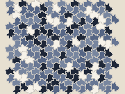
lizard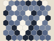
hex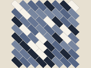
brick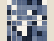
square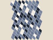
quad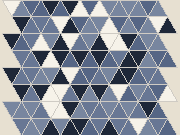
triangle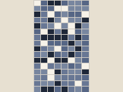
glide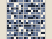
fourfold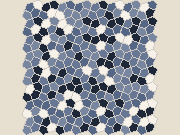
cairo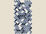
herring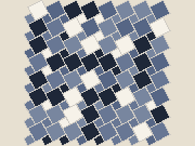
pythThe tile families of this page with their default shapes and JETCARP ids. Herringbone and the Pythagorean tiling are fixed; the others can be reshaped. Thumbnails from the tiling catalogue.
What it is
Each editable family is one prototile, a tile shape, together with rules for how its edges fit against its neighbours’. An edge can be paired with another edge by a slide (translation), by a turn about a shared corner, or by a half turn about its own midpoint, and an edge can be any curve as long as its partner follows it. The families JETCARP offers:
| Id | Family | How the edges pair | Neighbours (edge / touch) |
|---|---|---|---|
lizard | Three-fold hexagon | each edge turns 120° about a shared corner onto its partner | 6 / 6 |
hex | Hexagon | three pairs of opposite edges, each related by a slide | 6 / 6 |
brick | Brick | a hexagon with straight angles at two corners | 6 / 6 |
square | Square (parallelogram) | two pairs of opposite edges, each related by a slide | 4 / 8 |
quad | Any quadrilateral | each edge turns 180° about its own midpoint | 4 / 8 |
triangle | Any triangle | as for the quadrilateral; six triangles meet at each corner | 3 / 12 |
glide | Glide rectangle | top and bottom edges pair by a flip and a slide, so neighbouring rows are mirror images | 4 / 8 |
fourfold | Four-fold square | edges turn 90° about two opposite corners, so tiles spin in fours | 4 / 8 |
cairo | Cairo pentagon | one half-turn edge and two pairs that turn 90° | 5 / 7 |
Two fixed patterns sit beside them. Herringbone (herring) lays rectangles in two orientations and
Pythagorean squares (pyth) mixes two sizes of square; neither is edge to edge, so JETCARP measures
which tiles touch from the geometry. Herringbone has the hexagon grid’s neighbour graph; in the
Pythagorean tiling, large squares touch eight tiles and small squares four, exactly as the octagons
and squares of 4.8.8 do, and its neighbour graph is that of 4.8.8.
So, for any rule that only counts neighbours, several of these families are familiar grids in disguise: the brick, herringbone and three-fold (lizard) tilings behave exactly as hexagons, the quadrilateral, glide and four-fold tilings as squares, and the Pythagorean tiling as 4.8.8. JETCARP’s survey of neighbour graphs confirmed this for both neighbourhoods (Findings). A pattern found on one of them is a pattern of the grid it copies, and is presented as such.
The neighbour graph depends on the family, not on the exact shape, so reshaping a tile changes how the world looks but not how a rule behaves. That makes these families a way to draw: run a rule, then bend the tiles into fish or lizards.
B2/S34H) in another drawing. Scene
docs/scenes/tilings/editable-lizard.json.Where it came from
Cairo pentagons. The tiling is named after its use as street paving in Cairo; R. H. Macmillan’s note of 1979 is the classic written source, and Frank Morgan went looking for surviving Cairo pavements in 2019 (Macmillan 1979; Morgan 2019). Earlier appearances include Harry Nisbet’s Grammar of Textile Design (1906), a 1909 US patent for pentagonal floor tiles by Herbert C. Moore, P. A. MacMahon’s New Mathematical Pastimes (1921), and notes by A. P. Rollett (1955) and J. A. Dunn (1971) (Nisbet 1906; Moore 1909; MacMahon 1921; Rollett 1955; Dunn 1971). Mathematically it is the dual of the snub square tiling, and its pentagon belongs to one of the families of convex pentagons that tile the plane surveyed by Doris Schattschneider (Schattschneider 1978). Carter Bays found a Life-like glider on it (Bays 2005), which Matej Kerekrety showed again as the “shrimp” (Kerekrety 2020).
Pythagorean tiling. Two sizes of square, named for the dissection proofs of Pythagoras’s theorem it carries: lay a square grid with the hypotenuse as its side over it, and the two squares are cut into pieces that make the larger one (Frederickson 1997; Nelsen 2003; Aguiló, Fiol and Fiol 2000).
Herringbone. Rectangles in two orientations; Grünbaum and Shephard list it among the isohedral tilings by quadrangles (Grünbaum and Shephard 1987).
Brick. Running bond, each course offset by half a brick. Its neighbour graph is the hexagonal one, which is why Wolfram describes two-cell rules on cells “arranged like hexagons or staggered bricks” (Wolfram 2002).
The three-fold hexagon. Tom McLean’s catalogue describes isohedral type IH7 in the same way as this family: a hexagon whose adjacent sides pair up, meeting at 120° (McLean). M. C. Escher drew lizards on a regular division of the plane in drawing no. 25 (1939), and used the same angular lizard in the lithograph Reptiles (1943) (Kersten 2018; Schattschneider 1990); we have not found a source that states drawing no. 25 is of type IH7, though the shapes agree.
How JETCARP runs it
The editable families came from JETCARP’s original prototype tiling editor and keep its edge rules.
In the app, Edit tile… lets you drag a tile’s corners and reshape its edges; every edge’s partner
follows, and JETCARP checks that tiles still interlock without gaps or overlaps. A tile can also be
pasted as JSON, and a scene records it in the tiling’s params and edges, so a reshaped world
replays exactly. Beyond these families, the periodic family takes any polygons in a repeating unit
cell, which the app’s unit-cell editor can draw; contact between them is measured from the geometry.
What is new here
Nothing. These are classical tilings and well-known tile families, presented so that any rule can run on them and the tiles can be reshaped while it runs. Results on the brick, herringbone, lizard, quadrilateral, glide, four-fold and Pythagorean tilings are results on the hexagonal, square or 4.8.8 tiling they copy.
Try it
- Quick Start: B2/S34 on Escher’s lizard tile, and the Tiling showcase entries for brick, any quadrilateral, any triangle, glide rectangle, four-fold square, Cairo pentagon, herringbone and Pythagorean squares.
- Open a lizard world in the app, start a rule, and drag the tile’s corners.
References
- Macmillan 1979; Morgan 2019; Nisbet 1906; Moore 1909; MacMahon 1921; Rollett 1955; Dunn 1971; Schattschneider 1978
- Bays 2005; Kerekrety 2020
- Frederickson 1997; Nelsen 2003; Aguiló, Fiol and Fiol 2000
- Grünbaum and Shephard 1987; Wolfram 2002
- McLean; Kersten 2018; Schattschneider 1990
Penrose tilings
Penrose tilings cover the plane with two tile shapes in a pattern that never repeats: no shift of the tiling, however large, maps it onto itself. Yet they are highly ordered, with five-fold symmetry everywhere at every scale. JETCARP builds both of Roger Penrose’s two-tile versions, kites and darts (P2) and thick and thin rhombs (P3), as exact finite patches of up to millions of tiles, and every rule runs on them.
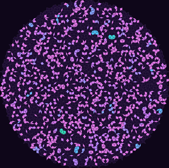
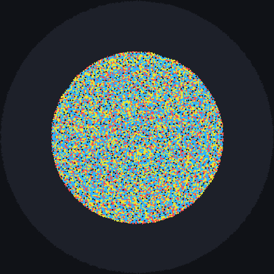
docs/scenes/tilings/penrose-rhomb-b2s34.json. Right:
30,000 sand grains dropped on a patch of Penrose kites and darts (P2) and toppled until stable; every
kite and dart has four edge neighbours, so all topple at four grains. Scene
docs/scenes/tilings/penrose-kd-sandpile.json.What it is
A tiling is aperiodic if no translation maps it onto itself and, more strongly, a set of tiles is aperiodic if every tiling it makes is non-periodic. Penrose’s tiles are such a set, with matching rules (marks on the edges, or notches) that forbid the periodic arrangements the bare shapes would allow:
- P2, kites and darts. Two quadrilaterals cut from a rhombus with angles of 72° and 108°. In a large patch, kites outnumber darts by the golden ratio φ ≈ 1.618.
- P3, rhombs. A thick rhomb (72° and 108°) and a thin one (36° and 144°), meeting edge to edge. Thick rhombs outnumber thin ones by φ.
Both can be built by deflation: cut every tile into smaller tiles of the same kinds, scale up, and repeat. Each Penrose tile splits into two mirror-image golden triangles (Robinson triangles), which deflate exactly, and this is how both tilings are usually generated.
For an automaton, a Penrose tiling is a neighbour graph in which every tile has four edge neighbours but a varying number of touch neighbours: 8 to 10 for kites and darts, 7 to 11 for rhombs. Because the graph never repeats, a pattern that moves meets a slightly different neighbourhood at every step, which is why gliders are so hard to find there.
Where it came from
Robert Berger showed in 1966 that the domino problem for Wang tiles is undecidable, which needed an aperiodic set of tiles (Berger 1966); Raphael M. Robinson simplified the construction in 1971 (Robinson 1971). Roger Penrose found much smaller aperiodic sets in the 1970s, reducing them to two tiles, the kite and dart and the two rhombs. Penrose’s US patent, “Set of tiles for covering a surface”, was filed in 1976 (with a UK priority date of June 1975) and granted in 1979 (Penrose 1979, patent); Penrose’s own account is “Pentaplexity” (Penrose 1979). Martin Gardner’s Scientific American column of January 1977 made the tilings widely known (Gardner 1977).
The Robinson triangles are named after Raphael Robinson; Grünbaum and Shephard give the standard account of them (Grünbaum and Shephard 1987, ch. 10). N. G. de Bruijn gave an algebraic theory of Penrose tilings in 1981 (de Bruijn 1981; part II). Jeff Preshing’s 2011 blog post explains generating them by triangle subdivision in a few lines of Python (Preshing 2011).
Cellular automata on Penrose tilings. Margaret Hill, Susan Stepney and Francis Wan studied the ash that Life leaves on Penrose tilings (Hill, Stepney and Wan 2005), and Nick Owens and Susan Stepney catalogued its still lifes and oscillators and found no gliders (Owens and Stepney 2010). Adam P. Goucher found the first glider that travels across an aperiodic tiling, in a four-state rule on a Penrose tiling (Goucher 2012). D. A. Bailey and K. A. Lindsey studied a Game of Life on Penrose tilings (Bailey and Lindsey 2017), Fersula, Noûs and Perrot computed sandpile identities on them (Fersula, Noûs and Perrot 2020), and Langton’s ant has been run on them (ptiles/ant).
How JETCARP runs it
JETCARP builds both tilings by exact Robinson-triangle deflation from a five-fold “sun” at the centre, pairing mirror-image triangles into whole tiles at the end; the code was written from the geometry of the triangles as Grünbaum and Shephard and de Bruijn describe it. Patches are chosen by level: level 3, 4 and 5 are the 500, 4,000 and 35,000 tiles nearest the centre, and levels 7 and 8 (about 2.2 and 18 million tiles) are built in exact integer coordinates, with every neighbour found by an exact lookup rather than a floating-point tolerance. Smaller patches nest inside larger ones. The tests check that there are no gaps or overlaps, that the vertex neighbourhoods are the legal Penrose ones (7 kinds for P2, 8 for P3), and that the tile ratios tend to φ.
In a scene: "tiling": {"family": "penrose-rhomb", "size": {"level": 4}} (or penrose-kd). Patch
edges are dead. Tiles are rigid copies of the two prototiles; their shapes cannot be edited.
What is new here
Cellular automata on Penrose tilings have a long history, summarised above, and we claim nothing new for the tilings themselves. JETCARP runs every family on them, including some (cyclic, Greenberg–Hastings, rock-paper-scissors, Hodgepodge and forest fire) for which our search found no earlier Penrose version; these are direct applications of known rules, so we do not count them as discoveries. JETCARP’s 71 JACA presets include several on both Penrose tilings.
Try it
- Quick Start: Sandpile on Penrose kites and darts, Brian’s Brain on Penrose rhombs, the Tiling showcase entries for both tilings, and JACA presets such as JACA rainbow fronts (Penrose rhombs).
jetcarp run docs/scenes/tilings/penrose-rhomb-b2s34.json --gens 200 --png rhombs.png
References
- Berger 1966; Robinson 1971
- Penrose 1979, patent; Penrose 1979; Gardner 1977
- Grünbaum and Shephard 1987; de Bruijn 1981; de Bruijn 1981, part II; Preshing 2011
- Hill, Stepney and Wan 2005; Owens and Stepney 2010; Goucher 2012; Bailey and Lindsey 2017; Fersula, Noûs and Perrot 2020; ptiles/ant
The hat and the spectre
Ever since the first aperiodic sets of tiles were found in the 1960s, mathematicians had asked whether a single tile could cover the plane only in patterns that never repeat: an einstein, from the German for “one stone”. In 2023 the answer came, twice in quick succession: the hat, found by a hobbyist, and then the spectre, which does it without ever needing its mirror image. JETCARP builds exact patches of both, up to about 18 million tiles, and runs every rule on them.
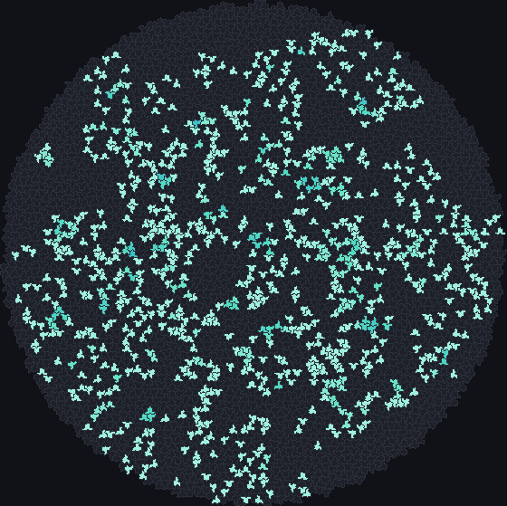
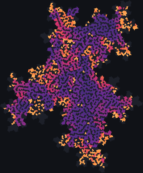
docs/scenes/tilings/hat-b2s34.json. Right: B2/S23 with edge neighbours on about 4,000
spectres, where each tile shares edges with four to seven others. Scene
docs/scenes/tilings/spectre-b2s23v.json. Both 200 generations.What it is
The hat is a polykite: eight of the kites of the Laves tiling [3.4.6.4], the tiling dual to 3.4.6.4, glued into a shape that looks a little like a hat or a shirt. Copies of it, together with some mirror-image copies, tile the plane, and every such tiling is non-periodic. The mirror-image hats are sparse; in JETCARP’s patches about one hat in eight is reflected, and the ratio of the two kinds tends to φ⁴ in large patches. The hat is one member of a continuous family of shapes, all aperiodic apart from three special cases.
The spectre comes from one of those special cases, the equilateral member of the family. Tiled without reflections it is aperiodic; changing its straight edges to curves gives the spectres, which tile only non-periodically and never use a mirror image, even when reflections are allowed. Its tilings follow a hierarchical substitution: groups of spectres form larger “supertiles” that fit together like spectres again.
For an automaton, both are neighbour graphs with no repeating structure. Each hat has 4 to 6 edge neighbours and 6 or 7 touch neighbours; each spectre 4 to 7 edge neighbours and 6 or 7 touch neighbours. The irregularity is mild, which is why rules made for hexagons often feel at home on the hat, yet movers face a different neighbourhood at every step.

docs/scenes/automata/priority-hat-glider.json. Right: a 4-cell oscillator with period 6
in B2567/S456, found by JETCARP's soup search. On an aperiodic tiling an oscillator is tied
to the cluster of tiles it sits on. Scene docs/scenes/tilings/osc-hat-p6.json.Where it came from
Earlier aperiodic sets needed more than one tile: Robert Berger’s first used thousands of Wang tiles, Roger Penrose’s used two (Berger 1966; see Penrose tilings). Joshua Socolar and Joan Taylor gave a single hexagonal tile that is aperiodic when combined with matching rules (Socolar and Taylor 2011).
David Smith, a hobbyist in Yorkshire, England, found the hat in the autumn of 2022, working largely by hand with the help of Jaap Scherphuis’s PolyForm Puzzle Solver, and emailed Craig S. Kaplan to ask that the shape be studied with Kaplan’s software (University of Waterloo 2023). Smith, Joseph Samuel Myers, Kaplan and Chaim Goodman-Strauss posted “An aperiodic monotile” in March 2023, and it was published in Combinatorial Theory in 2024. Their proof groups hats into four metatiles with a substitution rule (Smith et al. 2023). Two months later the same four authors showed in “A chiral aperiodic monotile” that the equilateral member of the family is aperiodic without reflections, and introduced the spectres (Smith et al. 2023b). Kaplan published software for both: hatviz, which builds hat patches from the metatile substitution, and an interactive spectre app (hatviz; hat page; spectre page).
Cellular automata on the monotiles. Within weeks of the hat’s announcement, Andrew Trevorrow’s HatLife ran Life-like, Larger than Life-style, WireWorld and “Worms” rules on it (Trevorrow 2023). James Edmond found gliders on both tiles in 2026, by evolutionary search over priority tables (Edmond 2026; see Priority rules and the Spectre glider).
How JETCARP runs it
JETCARP’s hat construction is ported from Kaplan’s hatviz, and its spectre construction from Kaplan’s spectre app, both under the BSD 3-Clause licence (Kaplan granted that licence for the spectre code to JETCARP in November 2026); the notices are in JETCARP’s third-party notices file. Patches are chosen by level: for the hat, levels 3, 4 and 5 are the 500, 4,000 and 35,000 tiles nearest a fixed centre, which is a reflected hat; for the spectre, a level is a supertile level of the substitution (about 4,400 tiles at level 4 and 35,000 at level 5). Levels 7 and 8, with about 2 million and 17 to 18 million tiles, are built in exact integer coordinates, and every neighbour is found by an exact lookup. The tests check for gaps and overlaps and that the hat to reflected-hat ratio tends to φ⁴.
In a scene: "tiling": {"family": "hat", "size": {"level": 4}} (or spectre). Patch edges are dead,
and the tile shapes are fixed. For movers that need more room than any patch,
jetcarp search mover can follow a pattern on a sliding window that builds supertiles around it
as it goes; JETCARP has followed the Spectre glider pair this way for 10 million rings of tiles.
What is new here
The tiles are Smith, Myers, Kaplan and Goodman-Strauss’s, and cellular automata on them began with Trevorrow and Edmond. JETCARP adds two things that, to our knowledge, have not been done before: it runs every rule family on the hat and spectre, including families (turmites, cyclic, Greenberg–Hastings, rock-paper-scissors, Hodgepodge, forest fire) for which our search found no earlier monotile version, though we count those only as direct applications; and it computes sandpile identities and large single-source sandpiles on both monotiles, where our search found no earlier sandpile work at all (see The Abelian sandpile and What is new in JETCARP). The hat glider found by JETCARP’s search is James Edmond’s hat glider B with its states renamed, and the credit is Edmond’s; JETCARP adds only a check that it runs for a million rings of tiles on a sliding window (see Priority rules).
Try it
- Quick Start: B2/S34 on the hat, Sandpile on the Spectre, Spectre glider, Layered parity on the Spectre, JACA war on the hat tiling, and the Tiling showcase entries for both tiles.
jetcarp run docs/scenes/tilings/hat-b2s34.json --gens 200 --png hat.pngjetcarp pile --tiling spectre --grains 1e6builds a million-grain sandpile on an exact spectre patch.
References
- Berger 1966; Socolar and Taylor 2011
- Smith et al. 2023; Smith et al. 2023b; University of Waterloo 2023
- hatviz; Kaplan, hat page; Kaplan, spectre page
- Trevorrow 2023; Edmond 2026
Tiling catalogue
Generated page. Built by
docs/tools/gen-tiling-catalogue.pyfrom the program’s own tiling lists and data files; thumbnails are drawn by JETCARP (docs/tools/tiling-thumbs.rhai). Do not edit by hand.
Every tiling JETCARP can run, with its neighbour counts. That is 25 tiling families (some of them reshapeable), 81 isohedral types, and the 1248 k-uniform tilings of Galebach’s catalogue, which include the regular and Archimedean tilings again under their catalogue ids.
How to read the degrees. A tile’s edge neighbours share a side with it; its touch neighbours share at least one corner (see Tilings as neighbour graphs). The lists give every value that occurs in the interior of the tiling. Rules that count neighbours (Life-like, Generations, JACA and others) see these numbers, which is why the same rule behaves so differently from one tiling to the next.
Thumbnails show a small patch with each tile in a random colour so the shapes stand out. Reshapeable families and isohedral types are drawn with their default shapes.
Tiling families
These are the families you pick by name (tiling: {"family": "cairo"} in a scene). Symmetry is the wallpaper group of the default shape (none for the aperiodic tilings). Storage is how JETCARP holds the cells: dense for a plain lattice, periodic for a repeating unit cell, explicit for a finite aperiodic patch.
| Id | Name | Symmetry | Storage | Edge degrees | Touch degrees | |
|---|---|---|---|---|---|---|
| lizard | Three-fold hexagon | p3 | periodic | 6 | 6 |
| hex | Hexagon | p1 | dense | 6 | 6 |
| brick | Brick | p1 | dense | 6 | 6 |
| square | Square (parallelogram) | p1 | dense | 4 | 8 |
| quad | Any quadrilateral | p2 | periodic | 4 | 8 |
| triangle | Any triangle | p2 | periodic | 3 | 12 |
| glide | Glide rectangle | pg | periodic | 4 | 8 |
| fourfold | Four-fold square | p4 | periodic | 4 | 8 |
| cairo | Cairo pentagon | p4 | periodic | 5 | 7 |
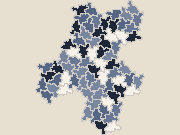 | spectre | Spectre | none | explicit | 4, 5, 6, 7 | 6, 7 |
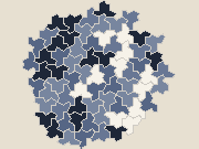 | hat | Hat | none | explicit | 4, 5, 6 | 6, 7 |
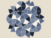 | penrose-kd | Penrose kites and darts (P2) | none | explicit | 4 | 8, 9, 10 |
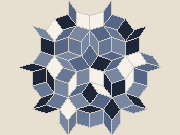 | penrose-rhomb | Penrose rhombs (P3) | none | explicit | 4 | 7, 8, 9, 10, 11 |
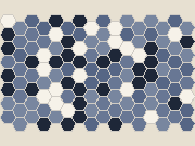 | hex_flat | Hexagon, flat top | p6m | periodic | 6 | 6 |
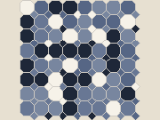 | oct | 4.8.8 truncated square | p4m | periodic | 4, 8 | 4, 8 |
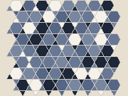 | trihex | 3.6.3.6 trihexagonal | p6m | periodic | 3, 6 | 6, 12 |
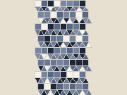 | elongtri | 3.3.3.4.4 elongated triangular | cmm | periodic | 3, 4 | 9, 12 |
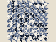 | snubsq | 3.3.4.3.4 snub square | p4g | periodic | 3, 4 | 9, 12 |
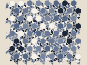 | snubhex | 3.3.3.3.6 snub hexagonal | p6 | periodic | 3, 6 | 9, 18 |
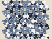 | rhombitrihex | 3.4.6.4 rhombitrihexagonal | p6m | periodic | 3, 4, 6 | 6, 8, 12 |
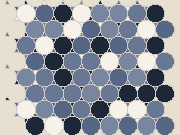 | trunchex | 3.12.12 truncated hexagonal | p6m | periodic | 3, 12 | 3, 12 |
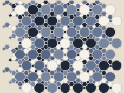 | trunctrihex | 4.6.12 truncated trihexagonal | p6m | periodic | 4, 6, 12 | 4, 6, 12 |
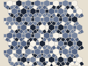 | periodic | Periodic (custom or catalog) | any | periodic | 3, 4, 6 | 6, 8, 12 |
| herring | Herringbone | pgg | periodic | 6 | 6 |
| pyth | Pythagorean squares | p4 | periodic | 4, 8 | 4, 8 |
Pages: Regular and Archimedean tilings, Editable tile families, Penrose tilings, The hat and the spectre.
Isohedral types
The 81 isohedral types that Craig Kaplan’s Tactile library supports (IH01 to IH93 in Grünbaum and Shephard’s numbering, less the 12 types Tactile does not support). Parameters is the number of shape sliders; aspects is the number of differently oriented copies of the tile in one unit cell. See Isohedral tilings.
| Id | Symmetry | Parameters | Aspects | Edge degrees | Touch degrees | |
|---|---|---|---|---|---|---|
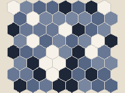 | ih01 | p1 | 4 | 1 | 6 | 6 |
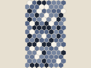 | ih02 | pg | 4 | 2 | 6 | 6 |
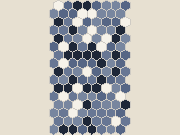 | ih03 | pg | 4 | 2 | 6 | 6 |
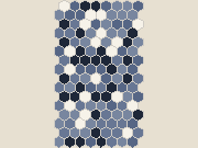 | ih04 | p2 | 6 | 2 | 6 | 6 |
 | ih05 | pgg | 5 | 4 | 6 | 6 |
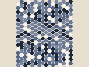 | ih06 | pgg | 5 | 4 | 6 | 6 |
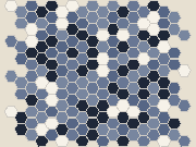 | ih07 | p3 | 2 | 3 | 6 | 6 |
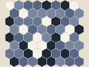 | ih08 | p2 | 4 | 1 | 6 | 6 |
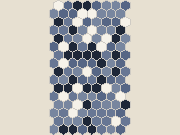 | ih09 | pgg | 3 | 2 | 6 | 6 |
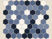 | ih10 | p3 | 0 | 1 | 6 | 6 |
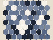 | ih11 | p6 | 0 | 1 | 6 | 6 |
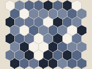 | ih12 | cm | 2 | 1 | 6 | 6 |
 | ih13 | pmg | 3 | 2 | 6 | 6 |
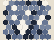 | ih14 | cm | 2 | 1 | 6 | 6 |
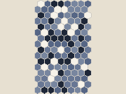 | ih15 | pmg | 3 | 2 | 6 | 6 |
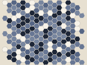 | ih16 | p31m | 1 | 3 | 6 | 6 |
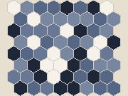 | ih17 | cmm | 2 | 1 | 6 | 6 |
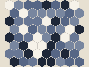 | ih18 | p31m | 0 | 1 | 6 | 6 |
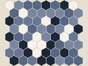 | ih20 | p6m | 0 | 1 | 6 | 6 |
 | ih21 | p6 | 2 | 6 | 5 | 8 |
 | ih22 | cm | 3 | 2 | 5 | 7 |
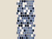 | ih23 | p2 | 4 | 2 | 5 | 7 |
 | ih24 | pmg | 4 | 4 | 5 | 7 |
 | ih25 | pgg | 3 | 4 | 5 | 7 |
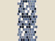 | ih26 | cmm | 2 | 2 | 5 | 7 |
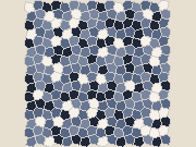 | ih27 | pgg | 3 | 4 | 5 | 7 |
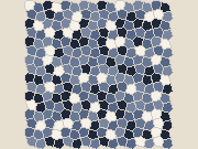 | ih28 | p4 | 2 | 4 | 5 | 7 |
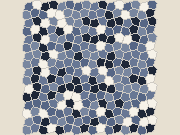 | ih29 | p4g | 1 | 4 | 5 | 7 |
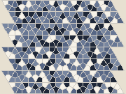 | ih30 | p31m | 1 | 6 | 4 | 9 |
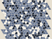 | ih31 | p6 | 0 | 6 | 4 | 9 |
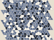 | ih32 | p6m | 0 | 6 | 4 | 9 |
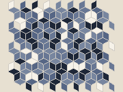 | ih33 | p3 | 0 | 3 | 4 | 10 |
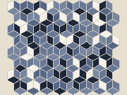 | ih34 | p6 | 0 | 3 | 4 | 10 |
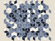 | ih36 | p31m | 0 | 3 | 4 | 10 |
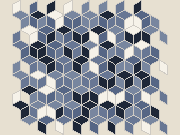 | ih37 | p6m | 0 | 3 | 4 | 10 |
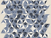 | ih38 | p31m | 0 | 6 | 3 | 21 |
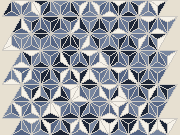 | ih39 | p6 | 0 | 6 | 3 | 21 |
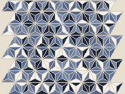 | ih40 | p6m | 0 | 6 | 3 | 21 |
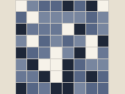 | ih41 | p1 | 2 | 1 | 4 | 8 |
 | ih42 | pm | 2 | 2 | 4 | 8 |
 | ih43 | pg | 2 | 2 | 4 | 8 |
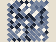 | ih44 | pg | 2 | 2 | 4 | 8 |
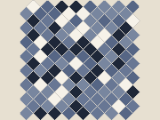 | ih45 | cm | 2 | 2 | 4 | 8 |
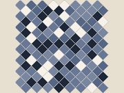 | ih46 | p2 | 4 | 2 | 4 | 8 |
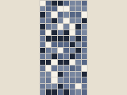 | ih47 | p2 | 2 | 2 | 4 | 8 |
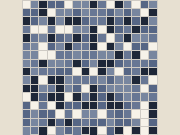 | ih49 | pmg | 3 | 4 | 4 | 8 |
 | ih50 | pmg | 2 | 4 | 4 | 8 |
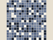 | ih51 | pgg | 3 | 4 | 4 | 8 |
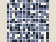 | ih52 | pgg | 1 | 4 | 4 | 8 |
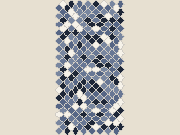 | ih53 | pgg | 3 | 4 | 4 | 8 |
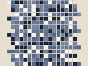 | ih54 | cmm | 2 | 4 | 4 | 8 |
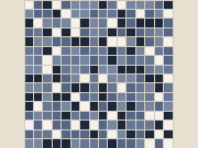 | ih55 | p4 | 0 | 4 | 4 | 8 |
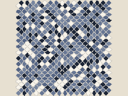 | ih56 | p4g | 1 | 8 | 4 | 8 |
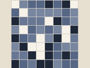 | ih57 | p2 | 2 | 1 | 4 | 8 |
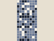 | ih58 | pmg | 2 | 2 | 4 | 8 |
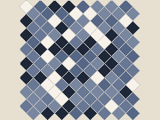 | ih59 | pgg | 1 | 2 | 4 | 8 |
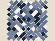 | ih61 | p4 | 0 | 2 | 4 | 8 |
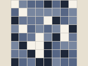 | ih62 | p4 | 0 | 1 | 4 | 8 |
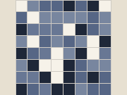 | ih64 | pm | 1 | 1 | 4 | 8 |
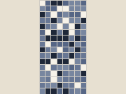 | ih66 | pmg | 1 | 2 | 4 | 8 |
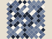 | ih67 | cmm | 2 | 2 | 4 | 8 |
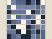 | ih68 | cm | 1 | 1 | 4 | 8 |
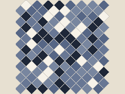 | ih69 | pmg | 2 | 2 | 4 | 8 |
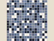 | ih71 | p4g | 0 | 4 | 4 | 8 |
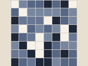 | ih72 | pmm | 1 | 1 | 4 | 8 |
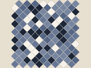 | ih73 | p4g | 0 | 2 | 4 | 8 |
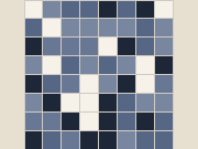 | ih74 | cmm | 1 | 1 | 4 | 8 |
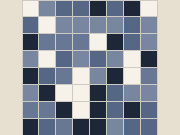 | ih76 | p4m | 0 | 1 | 4 | 8 |
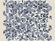 | ih77 | p6m | 0 | 12 | 3 | 16 |
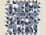 | ih78 | cmm | 1 | 4 | 3 | 14 |
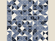 | ih79 | p4 | 0 | 4 | 3 | 14 |
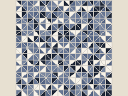 | ih81 | p4g | 0 | 8 | 3 | 14 |
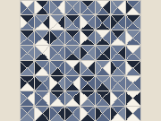 | ih82 | p4m | 0 | 4 | 3 | 14 |
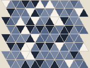 | ih83 | cm | 1 | 2 | 3 | 12 |
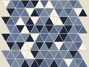 | ih84 | p2 | 2 | 2 | 3 | 12 |
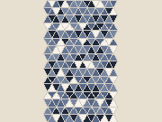 | ih85 | pmg | 2 | 4 | 3 | 12 |
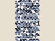 | ih86 | pgg | 1 | 4 | 3 | 12 |
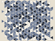 | ih88 | p6 | 0 | 6 | 3 | 12 |
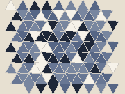 | ih90 | p6 | 0 | 2 | 3 | 12 |
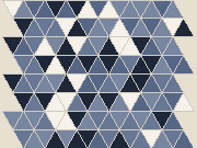 | ih91 | cmm | 1 | 2 | 3 | 12 |
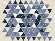 | ih93 | p6m | 0 | 2 | 3 | 12 |
k-uniform tilings, k = 1 to 3
Edge-to-edge tilings by regular polygons with k kinds of vertex (orbits under the tiling’s symmetries), from Brian Galebach’s catalogue in José Ezequiel Soto Sánchez’s encoding (CC BY 4.0). The name lists the vertex type of each orbit. Tiles is the number of tiles in one unit cell; mix is the share of each polygon; mean touch is the average touch degree over the tiles. k = 4 to 6 are on their own page. See k-uniform tilings.
Counts: k = 1: 11, k = 2: 20, k = 3: 61, k = 4: 151, k = 5: 332, k = 6: 673.
k = 1 (11 tilings)
| Id | Vertex types | Symmetry | Tiles | Mix | Edge degrees | Touch degrees | Mean touch | |
|---|---|---|---|---|---|---|---|---|
| k1-001 | 6^3 hexagonal | p6m | 1 | hexagons 100% | 6 | 6 | 6.00 |
| k1-002 | 4.8^2 truncated square | p4m | 2 | squares 50%, octagons 50% | 4, 8 | 4, 8 | 6.00 |
| k1-003 | 4.6.12 truncated trihexagonal | p6m | 6 | squares 50%, hexagons 33%, dodecagons 17% | 4, 6, 12 | 4, 6, 12 | 6.00 |
| k1-004 | 3.12^2 truncated hexagonal | p6m | 3 | triangles 67%, dodecagons 33% | 3, 12 | 3, 12 | 6.00 |
| k1-005 | 4^4 square | p4m | 1 | squares 100% | 4 | 8 | 8.00 |
| k1-006 | 3.4.6.4 rhombitrihexagonal | p6m | 6 | triangles 33%, squares 50%, hexagons 17% | 3, 4, 6 | 6, 8, 12 | 8.00 |
| k1-007 | 3.6.3.6 trihexagonal | p6m | 3 | triangles 67%, hexagons 33% | 3, 6 | 6, 12 | 8.00 |
| k1-008 | 3^3.4^2 elongated triangular | cmm | 3 | triangles 67%, squares 33% | 3, 4 | 9, 12 | 10.00 |
| k1-009 | 3^2.4.3.4 snub square | p4g | 6 | triangles 67%, squares 33% | 3, 4 | 9, 12 | 10.00 |
| k1-010 | 3^4.6 snub hexagonal | p6 | 9 | triangles 89%, hexagons 11% | 3, 6 | 9, 18 | 10.00 |
| k1-011 | 3^6 triangular | p6m | 2 | triangles 100% | 3 | 12 | 12.00 |
k = 2 (20 tilings)
| Id | Vertex types | Symmetry | Tiles | Mix | Edge degrees | Touch degrees | Mean touch | |
|---|---|---|---|---|---|---|---|---|
| k2-001 | [3.4.6.4; 4.6.12] | p6m | 12 | triangles 17%, squares 50%, hexagons 25%, dodecagons 8% | 3, 4, 6, 12 | 6, 8, 12 | 7.00 |
| k2-002 | [3.4.3.12; 3.12^2] | p4m | 6 | triangles 67%, squares 17%, dodecagons 17% | 3, 4, 12 | 5, 8, 16 | 7.33 |
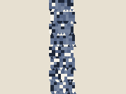 | k2-003 | [3^3.4^2; 4^4] #1 | cmm | 5 | triangles 40%, squares 60% | 3, 4 | 8, 9, 10 | 9.20 |
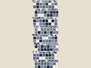 | k2-004 | [3^3.4^2; 4^4] #2 | cmm | 4 | triangles 50%, squares 50% | 3, 4 | 9, 10 | 9.50 |
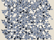 | k2-005 | [3.4^2.6; 3.4.6.4] | p6m | 18 | triangles 33%, squares 50%, hexagons 17% | 3, 4, 6 | 6, 8, 12 | 8.00 |
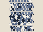 | k2-006 | [3.4^2.6; 3.6.3.6] #1 | cmm | 5 | triangles 40%, squares 40%, hexagons 20% | 3, 4, 6 | 6, 8, 12 | 8.00 |
| k2-007 | [3.4^2.6; 3.6.3.6] #2 | pmm | 5 | triangles 40%, squares 40%, hexagons 20% | 3, 4, 6 | 6, 8, 12 | 8.00 |
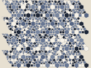 | k2-008 | [3^3.4^2; 3.4.6.4] | p6m | 15 | triangles 53%, squares 40%, hexagons 7% | 3, 4, 6 | 8, 9, 10, 12 | 9.20 |
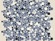 | k2-009 | [3^2.4.3.4; 3.4.6.4] | p6m | 15 | triangles 53%, squares 40%, hexagons 7% | 3, 4, 6 | 8, 9, 10, 12 | 9.20 |
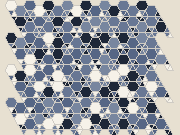 | k2-010 | [3^6; 3^2.6^2] | p6m | 8 | triangles 75%, hexagons 25% | 3, 6 | 8, 12 | 9.00 |
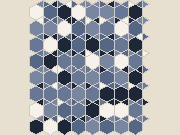 | k2-011 | [3^2.6^2; 3.6.3.6] | pmm | 3 | triangles 67%, hexagons 33% | 3, 6 | 6, 12 | 8.00 |
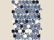 | k2-012 | [3^4.6; 3^2.6^2] | cmm | 5 | triangles 80%, hexagons 20% | 3, 6 | 8, 14 | 9.20 |
| k2-013 | [3^6; 3^2.4.12] | p6m | 16 | triangles 75%, squares 19%, dodecagons 6% | 3, 4, 12 | 8, 24 | 9.00 |
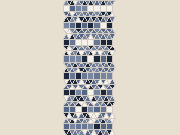 | k2-014 | [3^6; 3^3.4^2] #1 | pmm | 5 | triangles 80%, squares 20% | 3, 4 | 10, 11, 12 | 10.80 |
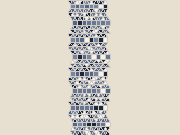 | k2-015 | [3^6; 3^3.4^2] #2 | cmm | 7 | triangles 86%, squares 14% | 3, 4 | 10, 11, 12 | 11.14 |
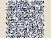 | k2-016 | [3^3.4^2; 3^2.4.3.4] #1 | p4g | 18 | triangles 67%, squares 33% | 3, 4 | 9, 12 | 10.00 |
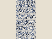 | k2-017 | [3^3.4^2; 3^2.4.3.4] #2 | pgg | 12 | triangles 67%, squares 33% | 3, 4 | 9, 12 | 10.00 |
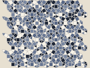 | k2-018 | [3^6; 3^2.4.3.4] | p6m | 11 | triangles 73%, squares 27% | 3, 4 | 9, 10, 12 | 10.36 |
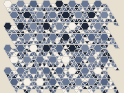 | k2-019 | [3^6; 3^4.6] #1 | p6m | 13 | triangles 92%, hexagons 8% | 3, 6 | 10, 18 | 10.62 |
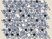 | k2-020 | [3^6; 3^4.6] #2 | p6 | 21 | triangles 95%, hexagons 5% | 3, 6 | 10, 11, 12, 18 | 11.14 |
k = 3 (61 tilings)
| Id | Vertex types | Symmetry | Tiles | Mix | Edge degrees | Touch degrees | Mean touch | |
|---|---|---|---|---|---|---|---|---|
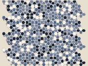 | k3-001 | [3^2.6^2; 3.6.3.6; 6^3] #1 | p6m | 15 | triangles 53%, hexagons 47% | 3, 6 | 6, 10 | 7.60 |
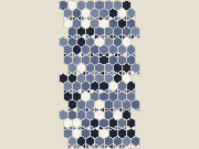 | k3-002 | [3^2.6^2; 3.6.3.6; 6^3] #2 | cmm | 4 | triangles 50%, hexagons 50% | 3, 6 | 6, 9 | 7.50 |
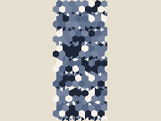 | k3-003 | [3^4.6; 3^2.6^2; 6^3] | pmg | 6 | triangles 67%, hexagons 33% | 3, 6 | 8, 10 | 8.67 |
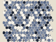 | k3-004 | [3^6; 3^2.6^2; 6^3] | p6m | 9 | triangles 67%, hexagons 33% | 3, 6 | 8, 10 | 8.67 |
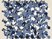 | k3-005 | [3.4^2.6; 3.6.3.6; 4.6.12] | p6m | 24 | triangles 33%, squares 38%, hexagons 25%, dodecagons 4% | 3, 4, 6, 12 | 6, 8, 10, 12 | 7.50 |
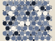 | k3-006 | [3^6; 3^2.4.12; 4.6.12] | p3m1 | 11 | triangles 55%, squares 27%, hexagons 9%, dodecagons 9% | 3, 4, 6, 12 | 6, 8, 18 | 8.18 |
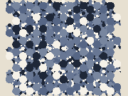 | k3-007 | [3^2.4.12; 3.4.6.4; 3.12^2] | p6m | 21 | triangles 57%, squares 29%, hexagons 5%, dodecagons 10% | 3, 4, 6, 12 | 5, 6, 8, 12, 18 | 7.71 |
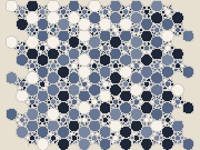 | k3-008 | [3.4.3.12; 3.4.6.4; 3.12^2] | p6m | 21 | triangles 57%, squares 29%, hexagons 5%, dodecagons 10% | 3, 4, 6, 12 | 5, 6, 8, 12, 18 | 7.71 |
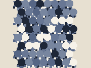 | k3-009 | [3^2.4.12; 3.4.3.12; 3.12^2] | cmm | 9 | triangles 67%, squares 22%, dodecagons 11% | 3, 4, 12 | 5, 6, 8, 20 | 7.78 |
 | k3-010 | [3^3.4^2; 4^4; 4^4] #1 | cmm | 7 | triangles 29%, squares 71% | 3, 4 | 8, 9, 10 | 8.86 |
| k3-011 | [3.4^2.6; 3.6.3.6; 4^4] #1 | cmm | 9 | triangles 22%, squares 67%, hexagons 11% | 3, 4, 6 | 6, 8, 12 | 8.00 |
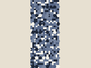 | k3-012 | [3.4^2.6; 3.6.3.6; 4^4] #2 | pmm | 9 | triangles 22%, squares 67%, hexagons 11% | 3, 4, 6 | 6, 8, 12 | 8.00 |
 | k3-013 | [3^3.4^2; 3^3.4^2; 4^4] #1 | pmm | 8 | triangles 50%, squares 50% | 3, 4 | 8, 9, 10, 12 | 9.50 |
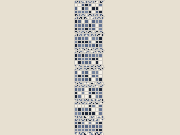 | k3-014 | [3^6; 3^3.4^2; 4^4] #1 | pmm | 7 | triangles 57%, squares 43% | 3, 4 | 8, 10, 11 | 10.00 |
 | k3-015 | [3^6; 3^3.4^2; 4^4] #2 | cmm | 9 | triangles 67%, squares 33% | 3, 4 | 8, 10, 11, 12 | 10.44 |
 | k3-016 | [3^3.4^2; 4^4; 4^4] #2 | cmm | 6 | triangles 33%, squares 67% | 3, 4 | 8, 9, 10 | 9.00 |
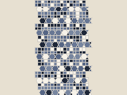 | k3-017 | [3.4^2.6; 3.6.3.6; 4^4] #3 | cmm | 7 | triangles 29%, squares 57%, hexagons 14% | 3, 4, 6 | 6, 8, 12 | 8.00 |
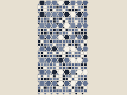 | k3-018 | [3.4^2.6; 3.6.3.6; 4^4] #4 | pmm | 7 | triangles 29%, squares 57%, hexagons 14% | 3, 4, 6 | 6, 8, 12 | 8.00 |
 | k3-019 | [3^3.4^2; 3^3.4^2; 4^4] #2 | pmm | 7 | triangles 57%, squares 43% | 3, 4 | 9, 10, 12 | 9.71 |
 | k3-020 | [3^6; 3^3.4^2; 4^4] #3 | pmm | 6 | triangles 67%, squares 33% | 3, 4 | 10, 11 | 10.33 |
 | k3-021 | [3^6; 3^3.4^2; 4^4] #4 | cmm | 8 | triangles 75%, squares 25% | 3, 4 | 10, 11, 12 | 10.75 |
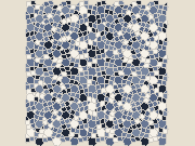 | k3-022 | [3.4^2.6; 3.4.6.4; 4^4] | p4g | 14 | triangles 29%, squares 57%, hexagons 14% | 3, 4, 6 | 6, 8, 12 | 8.00 |
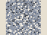 | k3-023 | [3^3.4^2; 3^2.4.3.4; 4^4] | p4 | 13 | triangles 62%, squares 38% | 3, 4 | 9, 11, 12 | 9.85 |
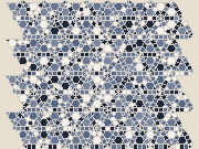 | k3-024 | [3^6; 3^2.4.3.4; 3.4^2.6] | p6m | 23 | triangles 52%, squares 39%, hexagons 9% | 3, 4, 6 | 7, 8, 10, 12 | 9.13 |
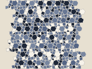 | k3-025 | [3^2.4.3.4; 3.4^2.6; 3.4.6.4] | cmm | 9 | triangles 44%, squares 44%, hexagons 11% | 3, 4, 6 | 7, 8, 9, 12 | 8.67 |
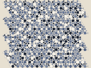 | k3-026 | [3.4^2.6; 3.4.6.4; 3.4.6.4] | p6m | 24 | triangles 33%, squares 50%, hexagons 17% | 3, 4, 6 | 6, 8, 12 | 8.00 |
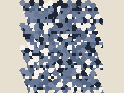 | k3-027 | [3^3.4^2; 3^2.6^2; 3.4^2.6] | cmm | 11 | triangles 55%, squares 27%, hexagons 18% | 3, 4, 6 | 7, 8, 10, 12 | 8.55 |
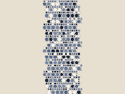 | k3-028 | [3.4^2.6; 3.4^2.6; 3.6.3.6] | cmm | 10 | triangles 40%, squares 40%, hexagons 20% | 3, 4, 6 | 6, 8, 12 | 8.00 |
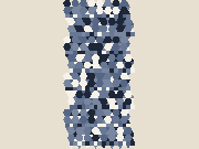 | k3-029 | [3^2.6^2; 3.4^2.6; 3.6.3.6] #1 | cmm | 8 | triangles 50%, squares 25%, hexagons 25% | 3, 4, 6 | 6, 8, 12 | 8.00 |
| k3-030 | [3.4^2.6; 3.6.3.6; 3.6.3.6] #1 | pmg | 8 | triangles 50%, squares 25%, hexagons 25% | 3, 4, 6 | 6, 8, 12 | 8.00 |
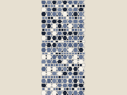 | k3-031 | [3^2.6^2; 3.4^2.6; 3.6.3.6] #2 | pmm | 8 | triangles 50%, squares 25%, hexagons 25% | 3, 4, 6 | 6, 8, 12 | 8.00 |
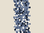 | k3-032 | [3.4^2.6; 3.6.3.6; 3.6.3.6] #2 | cmm | 8 | triangles 50%, squares 25%, hexagons 25% | 3, 4, 6 | 6, 8, 12 | 8.00 |
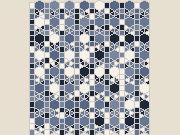 | k3-033 | [3^4.6; 3^3.4^2; 3.4^2.6] | pmm | 10 | triangles 60%, squares 30%, hexagons 10% | 3, 4, 6 | 8, 9, 10, 14 | 9.20 |
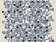 | k3-034 | [3^6; 3^2.4.3.4; 3.4.6.4] #1 | p6m | 23 | triangles 52%, squares 39%, hexagons 9% | 3, 4, 6 | 7, 8, 10, 12 | 9.13 |
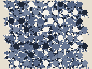 | k3-035 | [3^3.4^2; 3^2.4.12; 3.4.6.4] | p6m | 33 | triangles 55%, squares 36%, hexagons 6%, dodecagons 3% | 3, 4, 6, 12 | 7, 8, 10, 12, 24 | 8.55 |
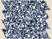 | k3-036 | [3^6; 3^3.4^2; 3.4.6.4] | p6m | 28 | triangles 64%, squares 32%, hexagons 4% | 3, 4, 6 | 8, 10, 12 | 9.86 |
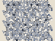 | k3-037 | [3^6; 3^2.4.3.4; 3.4.6.4] #2 | p6m | 28 | triangles 64%, squares 32%, hexagons 4% | 3, 4, 6 | 8, 10, 12 | 9.86 |
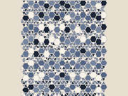 | k3-038 | [3^6; 3^4.6; 3^2.6^2] #1 | pmg | 14 | triangles 86%, hexagons 14% | 3, 6 | 8, 9, 10, 14 | 10.00 |
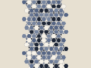 | k3-039 | [3^2.6^2; 3.6.3.6; 3.6.3.6] | cmm | 6 | triangles 67%, hexagons 33% | 3, 6 | 6, 12 | 8.00 |
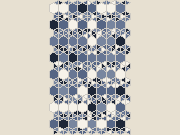 | k3-040 | [3^6; 3^4.6; 3^2.6^2] #2 | pmm | 7 | triangles 86%, hexagons 14% | 3, 6 | 9, 10, 14 | 10.00 |
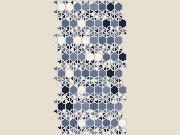 | k3-041 | [3^6; 3^4.6; 3^2.6^2] #3 | cmm | 9 | triangles 89%, hexagons 11% | 3, 6 | 9, 11, 14 | 10.44 |
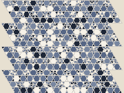 | k3-042 | [3^6; 3^4.6; 3.6.3.6] #1 | p6m | 17 | triangles 82%, hexagons 18% | 3, 6 | 6, 8, 10, 14 | 9.53 |
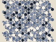 | k3-043 | [3^6; 3^4.6; 3.6.3.6] #2 | p6m | 14 | triangles 86%, hexagons 14% | 3, 6 | 8, 10, 15 | 9.86 |
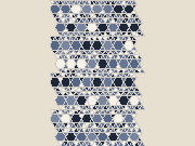 | k3-044 | [3^6; 3^4.6; 3.6.3.6] #3 | cmm | 11 | triangles 91%, hexagons 9% | 3, 6 | 8, 10, 11, 16 | 10.55 |
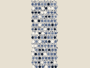 | k3-045 | [3^4.6; 3^4.6; 3.6.3.6] #1 | pmg | 14 | triangles 86%, hexagons 14% | 3, 6 | 8, 9, 16 | 9.71 |
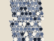 | k3-046 | [3^4.6; 3^4.6; 3.6.3.6] #2 | p2 | 7 | triangles 86%, hexagons 14% | 3, 6 | 8, 9, 16 | 9.71 |
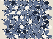 | k3-047 | [3^6; 3^3.4^2; 3^2.4.12] | p6m | 33 | triangles 79%, squares 18%, dodecagons 3% | 3, 4, 12 | 8, 9, 10, 11, 12, 24 | 10.00 |
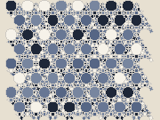 | k3-048 | [3^6; 3^2.4.3.4; 3^2.4.12] | p6m | 27 | triangles 74%, squares 22%, dodecagons 4% | 3, 4, 12 | 8, 9, 10, 24 | 9.56 |
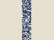 | k3-049 | [3^6; 3^6; 3^3.4^2] #1 | pmm | 9 | triangles 89%, squares 11% | 3, 4 | 10, 11, 12 | 11.33 |
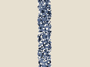 | k3-050 | [3^6; 3^6; 3^3.4^2] #2 | cmm | 11 | triangles 91%, squares 9% | 3, 4 | 10, 11, 12 | 11.45 |
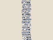 | k3-051 | [3^6; 3^3.4^2; 3^3.4^2] #1 | cmm | 8 | triangles 75%, squares 25% | 3, 4 | 9, 10, 11, 12 | 10.50 |
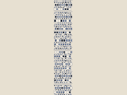 | k3-052 | [3^6; 3^3.4^2; 3^3.4^2] #2 | pmg | 10 | triangles 80%, squares 20% | 3, 4 | 9, 10, 11, 12 | 10.80 |
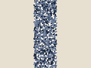 | k3-053 | [3^3.4^2; 3^3.4^2; 3^2.4.3.4] | pgg | 18 | triangles 67%, squares 33% | 3, 4 | 9, 12 | 10.00 |
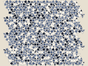 | k3-054 | [3^6; 3^3.4^2; 3^2.4.3.4] | p6m | 20 | triangles 70%, squares 30% | 3, 4 | 9, 10, 12 | 10.20 |
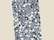 | k3-055 | [3^3.4^2; 3^2.4.3.4; 3^2.4.3.4] | p2 | 9 | triangles 67%, squares 33% | 3, 4 | 9, 12 | 10.00 |
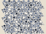 | k3-056 | [3^4.6; 3^3.4^2; 3^2.4.3.4] | p6m | 27 | triangles 74%, squares 22%, hexagons 4% | 3, 4, 6 | 9, 12, 18 | 10.00 |
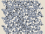 | k3-057 | [3^6; 3^2.4.3.4; 3^2.4.3.4] | p6m | 20 | triangles 70%, squares 30% | 3, 4 | 9, 10, 12 | 10.20 |
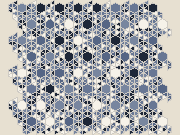 | k3-058 | [3^6; 3^6; 3^4.6] #1 | p6m | 19 | triangles 95%, hexagons 5% | 3, 6 | 10, 11, 18 | 11.05 |
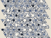 | k3-059 | [3^6; 3^6; 3^4.6] #2 | p6m | 27 | triangles 96%, hexagons 4% | 3, 6 | 10, 11, 12, 18 | 11.33 |
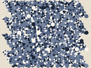 | k3-060 | [3^6; 3^6; 3^4.6] #3 | p6 | 33 | triangles 97%, hexagons 3% | 3, 6 | 10, 11, 12, 18 | 11.45 |
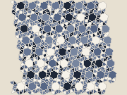 | k3-061 | [3^6; 3^4.6; 3^4.6] | cmm | 11 | triangles 91%, hexagons 9% | 3, 6 | 9, 10, 18 | 10.36 |
k-uniform tilings, k = 4 to 6
Generated page. Built by
docs/tools/gen-tiling-catalogue.pyfrom the program’s own tiling lists and data files; thumbnails are drawn by JETCARP (docs/tools/tiling-thumbs.rhai). Do not edit by hand.
The rest of Galebach’s catalogue, without thumbnails to keep the book small. To see one, run it: jetcarp script with world(#{ tiling: "k5-058" }), or pick it in the app’s Tiling catalog. Columns as on the main catalogue page.
k = 4 (151 tilings)
| Id | Vertex types | Symmetry | Tiles | Mix | Edge degrees | Touch degrees | Mean touch |
|---|---|---|---|---|---|---|---|
| k4-001 | [3^6; 3^2.6^2; 6^3; 6^3] #1 | p6m | 17 | triangles 35%, hexagons 65% | 3, 6 | 6, 8 | 7.41 |
| k4-002 | [3^6; 3^2.6^2; 6^3; 6^3] #2 | p6m | 22 | triangles 55%, hexagons 45% | 3, 6 | 6, 8, 10 | 8.18 |
| k4-003 | [3^3.4^2; 3^2.6^2; 3.4^2.6; 6^3] #1 | cmm | 13 | triangles 46%, squares 23%, hexagons 31% | 3, 4, 6 | 7, 8, 10 | 8.15 |
| k4-004 | [3^6; 3^2.6^2; 3^2.6^2; 6^3] #1 | cmm | 10 | triangles 60%, hexagons 40% | 3, 6 | 8, 10 | 8.40 |
| k4-005 | [3^6; 3^4.6; 3^2.6^2; 6^3] #1 | pmg | 16 | triangles 75%, hexagons 25% | 3, 6 | 8, 9, 10, 12 | 9.50 |
| k4-006 | [3^2.4.3.4; 3^2.6^2; 3.4^2.6; 6^3] | p6m | 30 | triangles 47%, squares 30%, hexagons 23% | 3, 4, 6 | 6, 7, 8, 9, 10 | 8.40 |
| k4-007 | [3^6; 3^2.6^2; 3^2.6^2; 6^3] #2 | p6m | 19 | triangles 63%, hexagons 37% | 3, 6 | 6, 8, 10 | 8.53 |
| k4-008 | [3^6; 3^2.6^2; 3^2.6^2; 6^3] #3 | p6m | 27 | triangles 67%, hexagons 33% | 3, 6 | 6, 8, 10, 12 | 8.67 |
| k4-009 | [3^4.6; 3^2.6^2; 3.6.3.6; 6^3] #1 | p6 | 21 | triangles 67%, hexagons 33% | 3, 6 | 6, 7, 8, 9, 11 | 8.57 |
| k4-010 | [3^4.6; 3^4.6; 3^2.6^2; 6^3] #1 | p6 | 27 | triangles 74%, hexagons 26% | 3, 6 | 6, 8, 9, 12 | 9.11 |
| k4-011 | [3^2.6^2; 3^2.6^2; 3.6.3.6; 6^3] | cmm | 7 | triangles 57%, hexagons 43% | 3, 6 | 6, 9, 12 | 7.71 |
| k4-012 | [3^6; 3^4.6; 3^2.6^2; 6^3] #2 | cmm | 8 | triangles 75%, hexagons 25% | 3, 6 | 9, 10 | 9.50 |
| k4-013 | [3^6; 3^4.6; 3^2.6^2; 6^3] #3 | pmg | 10 | triangles 80%, hexagons 20% | 3, 6 | 9, 10, 11 | 10.00 |
| k4-014 | [3^6; 3^2.6^2; 6^3; 6^3] #3 | p6m | 14 | triangles 43%, hexagons 57% | 3, 6 | 6, 8 | 7.71 |
| k4-015 | [3^2.6^2; 3.6.3.6; 6^3; 6^3] | pmm | 5 | triangles 40%, hexagons 60% | 3, 6 | 6, 9 | 7.20 |
| k4-016 | [3^4.6; 3^2.6^2; 6^3; 6^3] | cmm | 7 | triangles 57%, hexagons 43% | 3, 6 | 6, 8, 10 | 8.29 |
| k4-017 | [3^6; 3^2.6^2; 6^3; 6^3] #4 | p6 | 12 | triangles 50%, hexagons 50% | 3, 6 | 8 | 8.00 |
| k4-018 | [3^3.4^2; 3^2.6^2; 3.4^2.6; 6^3] #2 | pmm | 12 | triangles 50%, squares 25%, hexagons 25% | 3, 4, 6 | 7, 8, 10 | 8.33 |
| k4-019 | [3^6; 3^2.6^2; 3^2.6^2; 6^3] #4 | pmm | 9 | triangles 67%, hexagons 33% | 3, 6 | 8, 10 | 8.67 |
| k4-020 | [3^6; 3^4.6; 3^2.6^2; 6^3] #4 | cmm | 15 | triangles 80%, hexagons 20% | 3, 6 | 8, 9, 10, 12 | 9.73 |
| k4-021 | [3^2.6^2; 3.6.3.6; 3.6.3.6; 6^3] #1 | cmm | 10 | triangles 60%, hexagons 40% | 3, 6 | 6, 10, 11 | 7.80 |
| k4-022 | [3^2.6^2; 3.6.3.6; 3.6.3.6; 6^3] #2 | p6m | 19 | triangles 63%, hexagons 37% | 3, 6 | 6, 11, 12 | 7.89 |
| k4-023 | [3^4.6; 3^2.6^2; 3.6.3.6; 6^3] #2 | p3 | 11 | triangles 73%, hexagons 27% | 3, 6 | 6, 7, 8, 9, 12 | 8.73 |
| k4-024 | [3^4.6; 3^4.6; 3^2.6^2; 6^3] #2 | p31m | 17 | triangles 82%, hexagons 18% | 3, 6 | 8, 9, 14 | 9.53 |
| k4-025 | [3.4^2.6; 3.4^2.6; 3.4.6.4; 4.6.12] | p6m | 42 | triangles 29%, squares 50%, hexagons 19%, dodecagons 2% | 3, 4, 6, 12 | 6, 8, 10, 12 | 7.71 |
| k4-026 | [3^3.4^2; 3^2.6^2; 3.4^2.6; 4.6.12] | p6m | 39 | triangles 46%, squares 31%, hexagons 21%, dodecagons 3% | 3, 4, 6, 12 | 6, 7, 10, 12 | 8.15 |
| k4-027 | [3^2.4.3.4; 3^2.6^2; 3.4^2.6; 4.6.12] | p6m | 33 | triangles 42%, squares 36%, hexagons 18%, dodecagons 3% | 3, 4, 6, 12 | 6, 7, 9, 10, 12 | 8.18 |
| k4-028 | [3.4^2.6; 3.4.6.4; 4.6.12; 4.6.12] | p6m | 30 | triangles 20%, squares 50%, hexagons 23%, dodecagons 7% | 3, 4, 6, 12 | 4, 6, 8, 12 | 7.20 |
| k4-029 | [3.4.6.4; 3.4.6.4; 4.6.12; 4.6.12] | p6m | 30 | triangles 20%, squares 50%, hexagons 23%, dodecagons 7% | 3, 4, 6, 12 | 4, 6, 8, 12 | 7.20 |
| k4-030 | [3^2.4.12; 3.4.3.12; 3.4.6.4; 4.6.12] | cmm | 12 | triangles 50%, squares 33%, hexagons 8%, dodecagons 8% | 3, 4, 6, 12 | 6, 7, 8, 20 | 7.67 |
| k4-031 | [3^2.4.12; 3.4.6.4; 3.12^2; 3.12^2] | p6m | 24 | triangles 58%, squares 25%, hexagons 4%, dodecagons 12% | 3, 4, 6, 12 | 3, 5, 6, 8, 12, 16 | 7.50 |
| k4-032 | [3.4.3.12; 3.4.6.4; 3.12^2; 3.12^2] | p6m | 24 | triangles 58%, squares 25%, hexagons 4%, dodecagons 12% | 3, 4, 6, 12 | 3, 5, 6, 8, 12, 16 | 7.50 |
| k4-033 | [3.4.3.12; 3.12^2; 3.12^2; 3.12^2] | p4g | 18 | triangles 67%, squares 11%, dodecagons 22% | 3, 4, 12 | 3, 5, 8, 14 | 6.89 |
| k4-034 | [3^6; 3^2.4.3.4; 3^2.4.12; 3.12^2] | p6m | 26 | triangles 69%, squares 23%, dodecagons 8% | 3, 4, 12 | 5, 7, 10, 18 | 8.77 |
| k4-035 | [3^6; 3^2.4.3.4; 3.4.3.12; 3.12^2] | p6m | 26 | triangles 69%, squares 23%, dodecagons 8% | 3, 4, 12 | 5, 7, 10, 18 | 8.77 |
| k4-036 | [3^3.4^2; 3^2.4.12; 3.4.3.12; 3.12^2] #1 | pmm | 12 | triangles 67%, squares 25%, dodecagons 8% | 3, 4, 12 | 5, 7, 8, 10, 20 | 8.33 |
| k4-037 | [3^3.4^2; 3^2.4.12; 3.4.3.12; 3.12^2] #2 | cmm | 15 | triangles 67%, squares 27%, dodecagons 7% | 3, 4, 12 | 5, 7, 8, 10, 20 | 8.67 |
| k4-038 | [3^3.4^2; 4^4; 4^4; 4^4] #1 | cmm | 9 | triangles 22%, squares 78% | 3, 4 | 8, 9, 10 | 8.67 |
| k4-039 | [3.4^2.6; 3.6.3.6; 4^4; 4^4] #1 | cmm | 13 | triangles 15%, squares 77%, hexagons 8% | 3, 4, 6 | 6, 8, 12 | 8.00 |
| k4-040 | [3.4^2.6; 3.6.3.6; 4^4; 4^4] #2 | pmm | 13 | triangles 15%, squares 77%, hexagons 8% | 3, 4, 6 | 6, 8, 12 | 8.00 |
| k4-041 | [3^3.4^2; 3^3.4^2; 4^4; 4^4] #1 | pmm | 10 | triangles 40%, squares 60% | 3, 4 | 8, 9, 10, 12 | 9.20 |
| k4-042 | [3^6; 3^3.4^2; 4^4; 4^4] #1 | pmm | 9 | triangles 44%, squares 56% | 3, 4 | 8, 10, 11 | 9.56 |
| k4-043 | [3^6; 3^3.4^2; 4^4; 4^4] #2 | cmm | 11 | triangles 55%, squares 45% | 3, 4 | 8, 10, 11, 12 | 10.00 |
| k4-044 | [3.4^2.6; 3.4^2.6; 3.6.3.6; 4^4] #1 | cmm | 14 | triangles 29%, squares 57%, hexagons 14% | 3, 4, 6 | 6, 8, 12 | 8.00 |
| k4-045 | [3.4^2.6; 3.4^2.6; 3.6.3.6; 4^4] #2 | pmg | 14 | triangles 29%, squares 57%, hexagons 14% | 3, 4, 6 | 6, 8, 12 | 8.00 |
| k4-046 | [3^2.6^2; 3.4^2.6; 3.6.3.6; 4^4] #1 | cmm | 12 | triangles 33%, squares 50%, hexagons 17% | 3, 4, 6 | 6, 8, 12 | 8.00 |
| k4-047 | [3.4^2.6; 3.6.3.6; 3.6.3.6; 4^4] #1 | pmg | 12 | triangles 33%, squares 50%, hexagons 17% | 3, 4, 6 | 6, 8, 12 | 8.00 |
| k4-048 | [3.4^2.6; 3.4^2.6; 3.6.3.6; 4^4] #3 | pmm | 14 | triangles 29%, squares 57%, hexagons 14% | 3, 4, 6 | 6, 8, 12 | 8.00 |
| k4-049 | [3.4^2.6; 3.4^2.6; 3.6.3.6; 4^4] #4 | cmm | 14 | triangles 29%, squares 57%, hexagons 14% | 3, 4, 6 | 6, 8, 12 | 8.00 |
| k4-050 | [3^2.6^2; 3.4^2.6; 3.6.3.6; 4^4] #2 | pmm | 12 | triangles 33%, squares 50%, hexagons 17% | 3, 4, 6 | 6, 8, 12 | 8.00 |
| k4-051 | [3.4^2.6; 3.6.3.6; 3.6.3.6; 4^4] #2 | cmm | 12 | triangles 33%, squares 50%, hexagons 17% | 3, 4, 6 | 6, 8, 12 | 8.00 |
| k4-052 | [3^3.4^2; 3^3.4^2; 4^4; 4^4] #2 | pmm | 9 | triangles 44%, squares 56% | 3, 4 | 8, 9, 10 | 9.33 |
| k4-053 | [3^3.4^2; 3^3.4^2; 3^3.4^2; 4^4] #1 | cmm | 11 | triangles 55%, squares 45% | 3, 4 | 8, 9, 10, 12 | 9.64 |
| k4-054 | [3^6; 3^3.4^2; 3^3.4^2; 4^4] #1 | pmm | 12 | triangles 67%, squares 33% | 3, 4 | 8, 10, 11, 12 | 10.33 |
| k4-055 | [3^6; 3^6; 3^3.4^2; 4^4] #1 | pmm | 11 | triangles 73%, squares 27% | 3, 4 | 8, 10, 11, 12 | 10.73 |
| k4-056 | [3^6; 3^6; 3^3.4^2; 4^4] #2 | cmm | 13 | triangles 77%, squares 23% | 3, 4 | 8, 10, 11, 12 | 10.92 |
| k4-057 | [3^3.4^2; 3^3.4^2; 3^2.4.3.4; 4^4] #1 | p4 | 22 | triangles 55%, squares 45% | 3, 4 | 8, 9, 10, 11, 12 | 9.64 |
| k4-058 | [3^3.4^2; 4^4; 4^4; 4^4] #2 | cmm | 8 | triangles 25%, squares 75% | 3, 4 | 8, 9, 10 | 8.75 |
| k4-059 | [3.4^2.6; 3.6.3.6; 4^4; 4^4] #3 | cmm | 11 | triangles 18%, squares 73%, hexagons 9% | 3, 4, 6 | 6, 8, 12 | 8.00 |
| k4-060 | [3.4^2.6; 3.6.3.6; 4^4; 4^4] #4 | pmm | 11 | triangles 18%, squares 73%, hexagons 9% | 3, 4, 6 | 6, 8, 12 | 8.00 |
| k4-061 | [3^3.4^2; 3^3.4^2; 4^4; 4^4] #3 | pmm | 9 | triangles 44%, squares 56% | 3, 4 | 8, 9, 10, 12 | 9.33 |
| k4-062 | [3^6; 3^3.4^2; 4^4; 4^4] #3 | pmm | 8 | triangles 50%, squares 50% | 3, 4 | 8, 10, 11 | 9.75 |
| k4-063 | [3^6; 3^3.4^2; 4^4; 4^4] #4 | cmm | 10 | triangles 60%, squares 40% | 3, 4 | 8, 10, 11, 12 | 10.20 |
| k4-064 | [3.4^2.6; 3.4^2.6; 3.6.3.6; 4^4] #5 | cmm | 12 | triangles 33%, squares 50%, hexagons 17% | 3, 4, 6 | 6, 8, 12 | 8.00 |
| k4-065 | [3.4^2.6; 3.4^2.6; 3.6.3.6; 4^4] #6 | pmg | 12 | triangles 33%, squares 50%, hexagons 17% | 3, 4, 6 | 6, 8, 12 | 8.00 |
| k4-066 | [3^2.6^2; 3.4^2.6; 3.6.3.6; 4^4] #3 | cmm | 10 | triangles 40%, squares 40%, hexagons 20% | 3, 4, 6 | 6, 8, 12 | 8.00 |
| k4-067 | [3.4^2.6; 3.6.3.6; 3.6.3.6; 4^4] #3 | pmg | 10 | triangles 40%, squares 40%, hexagons 20% | 3, 4, 6 | 6, 8, 12 | 8.00 |
| k4-068 | [3.4^2.6; 3.4^2.6; 3.6.3.6; 4^4] #7 | pmm | 12 | triangles 33%, squares 50%, hexagons 17% | 3, 4, 6 | 6, 8, 12 | 8.00 |
| k4-069 | [3.4^2.6; 3.4^2.6; 3.6.3.6; 4^4] #8 | cmm | 12 | triangles 33%, squares 50%, hexagons 17% | 3, 4, 6 | 6, 8, 12 | 8.00 |
| k4-070 | [3^2.6^2; 3.4^2.6; 3.6.3.6; 4^4] #4 | pmm | 10 | triangles 40%, squares 40%, hexagons 20% | 3, 4, 6 | 6, 8, 12 | 8.00 |
| k4-071 | [3.4^2.6; 3.6.3.6; 3.6.3.6; 4^4] #4 | cmm | 10 | triangles 40%, squares 40%, hexagons 20% | 3, 4, 6 | 6, 8, 12 | 8.00 |
| k4-072 | [3^3.4^2; 3^3.4^2; 3^3.4^2; 4^4] #2 | cmm | 10 | triangles 60%, squares 40% | 3, 4 | 9, 10, 12 | 9.80 |
| k4-073 | [3^6; 3^3.4^2; 3^3.4^2; 4^4] #2 | pmm | 11 | triangles 73%, squares 27% | 3, 4 | 10, 11, 12 | 10.55 |
| k4-074 | [3^6; 3^6; 3^3.4^2; 4^4] #3 | pmm | 10 | triangles 80%, squares 20% | 3, 4 | 10, 11, 12 | 11.00 |
| k4-075 | [3^6; 3^6; 3^3.4^2; 4^4] #4 | cmm | 12 | triangles 83%, squares 17% | 3, 4 | 10, 11, 12 | 11.17 |
| k4-076 | [3^3.4^2; 3^3.4^2; 3^3.4^2; 4^4] #3 | cmm | 11 | triangles 55%, squares 45% | 3, 4 | 9, 10, 12 | 9.64 |
| k4-077 | [3^6; 3^3.4^2; 3^3.4^2; 4^4] #3 | cmm | 10 | triangles 60%, squares 40% | 3, 4 | 9, 10, 11 | 10.00 |
| k4-078 | [3^6; 3^3.4^2; 3^3.4^2; 4^4] #4 | pmg | 12 | triangles 67%, squares 33% | 3, 4 | 9, 10, 11, 12 | 10.33 |
| k4-079 | [3^3.4^2; 3^3.4^2; 3^2.4.3.4; 4^4] #2 | p4g | 34 | triangles 59%, squares 41% | 3, 4 | 9, 10, 11, 12 | 9.76 |
| k4-080 | [3.4^2.6; 3.4^2.6; 3.4.6.4; 4^4] | p4g | 26 | triangles 31%, squares 54%, hexagons 15% | 3, 4, 6 | 6, 8, 12 | 8.00 |
| k4-081 | [3^3.4^2; 3^2.4.12; 3.4.3.12; 4^4] | p4m | 19 | triangles 63%, squares 32%, dodecagons 5% | 3, 4, 12 | 7, 8, 10, 24 | 8.63 |
| k4-082 | [3^6; 3^3.4^2; 3^2.4.3.4; 4^4] | p4g | 24 | triangles 67%, squares 33% | 3, 4 | 9, 10, 11 | 10.17 |
| k4-083 | [3.4^2.6; 3.4^2.6; 3.4.6.4; 3.6.3.6] | p6m | 36 | triangles 39%, squares 42%, hexagons 19% | 3, 4, 6 | 6, 8, 12 | 8.00 |
| k4-084 | [3^6; 3^2.4.3.4; 3.4^2.6; 3.4.6.4] | p6m | 29 | triangles 48%, squares 41%, hexagons 10% | 3, 4, 6 | 6, 7, 8, 10, 12 | 8.90 |
| k4-085 | [3^2.4.3.4; 3^2.6^2; 3.4^2.6; 3.4.6.4] | cmm | 13 | triangles 46%, squares 38%, hexagons 15% | 3, 4, 6 | 7, 8, 9, 12 | 8.46 |
| k4-086 | [3^2.6^2; 3.4^2.6; 3.6.3.6; 3.6.3.6] #1 | cmm | 11 | triangles 55%, squares 18%, hexagons 27% | 3, 4, 6 | 6, 8, 12 | 8.00 |
| k4-087 | [3.4^2.6; 3.6.3.6; 3.6.3.6; 3.6.3.6] #1 | cmm | 11 | triangles 55%, squares 18%, hexagons 27% | 3, 4, 6 | 6, 8, 12 | 8.00 |
| k4-088 | [3^6; 3^4.6; 3.4^2.6; 3.6.3.6] #1 | pmg | 16 | triangles 75%, squares 12%, hexagons 12% | 3, 4, 6 | 6, 8, 10, 11, 14 | 9.75 |
| k4-089 | [3^2.6^2; 3.4^2.6; 3.6.3.6; 3.6.3.6] #2 | pmm | 11 | triangles 55%, squares 18%, hexagons 27% | 3, 4, 6 | 6, 8, 12 | 8.00 |
| k4-090 | [3.4^2.6; 3.6.3.6; 3.6.3.6; 3.6.3.6] #2 | pmm | 11 | triangles 55%, squares 18%, hexagons 27% | 3, 4, 6 | 6, 8, 12 | 8.00 |
| k4-091 | [3^6; 3^4.6; 3.4^2.6; 3.6.3.6] #2 | cmm | 16 | triangles 75%, squares 12%, hexagons 12% | 3, 4, 6 | 6, 8, 10, 11, 14 | 9.75 |
| k4-092 | [3^6; 3^3.4^2; 3.4^2.6; 3.6.3.6] | cmm | 15 | triangles 67%, squares 27%, hexagons 7% | 3, 4, 6 | 6, 10, 11, 12 | 9.87 |
| k4-093 | [3.4^2.6; 3.4.6.4; 3.4.6.4; 3.6.3.6] #1 | cmm | 11 | triangles 36%, squares 45%, hexagons 18% | 3, 4, 6 | 6, 8, 12 | 8.00 |
| k4-094 | [3.4^2.6; 3.4.6.4; 3.4.6.4; 3.6.3.6] #2 | p6m | 36 | triangles 39%, squares 42%, hexagons 19% | 3, 4, 6 | 6, 8, 12 | 8.00 |
| k4-095 | [3.4^2.6; 3.4.6.4; 3.6.3.6; 3.6.3.6] | p6m | 30 | triangles 47%, squares 30%, hexagons 23% | 3, 4, 6 | 6, 8, 12 | 8.00 |
| k4-096 | [3^6; 3^4.6; 3^3.4^2; 3.4^2.6] #1 | pmm | 15 | triangles 67%, squares 27%, hexagons 7% | 3, 4, 6 | 8, 10, 12, 14 | 9.73 |
| k4-097 | [3^4.6; 3^2.4.3.4; 3^2.4.3.4; 3.4^2.6] | cmm | 16 | triangles 62%, squares 31%, hexagons 6% | 3, 4, 6 | 8, 9, 10, 12, 14 | 9.50 |
| k4-098 | [3^6; 3^4.6; 3^3.4^2; 3.4^2.6] #2 | cmm | 15 | triangles 67%, squares 27%, hexagons 7% | 3, 4, 6 | 8, 10, 14 | 9.73 |
| k4-099 | [3^4.6; 3^3.4^2; 3.4^2.6; 3.4^2.6] | p2 | 10 | triangles 60%, squares 30%, hexagons 10% | 3, 4, 6 | 8, 9, 10, 14 | 9.20 |
| k4-100 | [3^6; 3^3.4^2; 3^3.4^2; 3.4.6.4] | p6m | 45 | triangles 71%, squares 27%, hexagons 2% | 3, 4, 6 | 8, 10, 11, 12 | 10.27 |
| k4-101 | [3^6; 3^3.4^2; 3^2.4.3.4; 3.4.6.4] #1 | p6m | 39 | triangles 67%, squares 31%, hexagons 3% | 3, 4, 6 | 8, 9, 10, 12 | 10.00 |
| k4-102 | [3^3.4^2; 3^2.4.3.4; 3.4.6.4; 3.4.6.4] | p6m | 45 | triangles 53%, squares 40%, hexagons 7% | 3, 4, 6 | 8, 9, 10, 12 | 9.20 |
| k4-103 | [3^6; 3^3.4^2; 3^2.4.3.4; 3.4.6.4] #2 | p6m | 45 | triangles 71%, squares 27%, hexagons 2% | 3, 4, 6 | 8, 10, 11, 12 | 10.27 |
| k4-104 | [3^6; 3^2.4.3.4; 3^2.4.3.4; 3.4.6.4] | p6m | 39 | triangles 67%, squares 31%, hexagons 3% | 3, 4, 6 | 8, 9, 10, 12 | 10.00 |
| k4-105 | [3^6; 3^2.4.3.4; 3.4.6.4; 3.4.6.4] | p6m | 29 | triangles 48%, squares 41%, hexagons 10% | 3, 4, 6 | 6, 7, 8, 10, 12 | 8.90 |
| k4-106 | [3^2.4.3.4; 3^2.4.3.4; 3.4.6.4; 3.4.6.4] #1 | pmm | 12 | triangles 50%, squares 42%, hexagons 8% | 3, 4, 6 | 7, 8, 9, 10, 12 | 9.00 |
| k4-107 | [3^2.4.3.4; 3^2.4.3.4; 3.4.6.4; 3.4.6.4] #2 | p4g | 36 | triangles 56%, squares 39%, hexagons 6% | 3, 4, 6 | 8, 9, 10, 12 | 9.33 |
| k4-108 | [3^2.4.3.4; 3.4.3.12; 3.4.6.4; 3.4.6.4] | p6m | 33 | triangles 55%, squares 36%, hexagons 6%, dodecagons 3% | 3, 4, 6, 12 | 6, 7, 8, 9, 12, 24 | 8.55 |
| k4-109 | [3^6; 3^4.6; 3^2.6^2; 3^2.6^2] | cmm | 15 | triangles 80%, hexagons 20% | 3, 6 | 8, 9, 10, 12, 14 | 9.47 |
| k4-110 | [3^6; 3^4.6; 3^4.6; 3^2.6^2] | p6m | 42 | triangles 86%, hexagons 14% | 3, 6 | 8, 9, 10, 12, 14, 18 | 10.00 |
| k4-111 | [3^6; 3^2.6^2; 3^2.6^2; 3.6.3.6] | p6m | 20 | triangles 70%, hexagons 30% | 3, 6 | 6, 8, 12 | 8.40 |
| k4-112 | [3^4.6; 3^2.6^2; 3^2.6^2; 3.6.3.6] #1 | p2 | 8 | triangles 75%, hexagons 25% | 3, 6 | 7, 8, 13 | 8.75 |
| k4-113 | [3^4.6; 3^2.6^2; 3^2.6^2; 3.6.3.6] #2 | pgg | 16 | triangles 75%, hexagons 25% | 3, 6 | 7, 8, 13 | 8.75 |
| k4-114 | [3^2.6^2; 3.6.3.6; 3.6.3.6; 3.6.3.6] #1 | pmm | 9 | triangles 67%, hexagons 33% | 3, 6 | 6, 12 | 8.00 |
| k4-115 | [3^6; 3^4.6; 3^2.6^2; 3.6.3.6] | cmm | 14 | triangles 86%, hexagons 14% | 3, 6 | 6, 8, 10, 11, 14 | 10.00 |
| k4-116 | [3^4.6; 3^4.6; 3^2.6^2; 3.6.3.6] #1 | p2 | 10 | triangles 80%, hexagons 20% | 3, 6 | 6, 8, 9, 14 | 9.20 |
| k4-117 | [3^2.6^2; 3.6.3.6; 3.6.3.6; 3.6.3.6] #2 | cmm | 9 | triangles 67%, hexagons 33% | 3, 6 | 6, 12 | 8.00 |
| k4-118 | [3^4.6; 3^2.6^2; 3.6.3.6; 3.6.3.6] #1 | p31m | 24 | triangles 75%, hexagons 25% | 3, 6 | 6, 7, 8, 9, 12, 14 | 8.75 |
| k4-119 | [3^4.6; 3^2.6^2; 3.6.3.6; 3.6.3.6] #2 | p6 | 27 | triangles 74%, hexagons 26% | 3, 6 | 6, 7, 8, 9, 12, 13 | 8.67 |
| k4-120 | [3^4.6; 3^4.6; 3^2.6^2; 3.6.3.6] #2 | pgg | 20 | triangles 80%, hexagons 20% | 3, 6 | 7, 8, 9, 14 | 9.20 |
| k4-121 | [3^4.6; 3^2.6^2; 3^2.6^2; 3.6.3.6] #3 | cmm | 8 | triangles 75%, hexagons 25% | 3, 6 | 6, 8, 13 | 8.75 |
| k4-122 | [3^6; 3^6; 3^4.6; 3^2.6^2] #1 | pmm | 11 | triangles 91%, hexagons 9% | 3, 6 | 9, 11, 12, 14 | 10.73 |
| k4-123 | [3^6; 3^6; 3^4.6; 3^2.6^2] #2 | cmm | 13 | triangles 92%, hexagons 8% | 3, 6 | 9, 11, 12, 14 | 10.92 |
| k4-124 | [3^6; 3^4.6; 3.6.3.6; 3.6.3.6] | pmg | 14 | triangles 86%, hexagons 14% | 3, 6 | 6, 8, 10, 11, 14 | 10.00 |
| k4-125 | [3^4.6; 3^4.6; 3.6.3.6; 3.6.3.6] | pgg | 20 | triangles 80%, hexagons 20% | 3, 6 | 6, 8, 9, 14 | 9.20 |
| k4-126 | [3^4.6; 3^3.4^2; 3^3.4^2; 3.6.3.6] #1 | pmm | 13 | triangles 77%, squares 15%, hexagons 8% | 3, 4, 6 | 8, 9, 12, 16 | 9.85 |
| k4-127 | [3^4.6; 3^3.4^2; 3^3.4^2; 3.6.3.6] #2 | cmm | 13 | triangles 77%, squares 15%, hexagons 8% | 3, 4, 6 | 8, 9, 12, 16 | 9.85 |
| k4-128 | [3^6; 3^6; 3^4.6; 3.6.3.6] | pmm | 11 | triangles 91%, hexagons 9% | 3, 6 | 8, 10, 11, 16 | 10.55 |
| k4-129 | [3^4.6; 3^4.6; 3^4.6; 3.6.3.6] | pmg | 14 | triangles 86%, hexagons 14% | 3, 6 | 8, 9, 16 | 9.71 |
| k4-130 | [3^6; 3^6; 3^3.4^2; 3^2.4.12] | p6m | 54 | triangles 81%, squares 17%, dodecagons 2% | 3, 4, 12 | 8, 9, 10, 11, 12, 24 | 10.44 |
| k4-131 | [3^6; 3^3.4^2; 3^2.4.3.4; 3^2.4.12] | p6m | 43 | triangles 70%, squares 28%, dodecagons 2% | 3, 4, 12 | 7, 8, 10, 12, 24 | 9.63 |
| k4-132 | [3^2.4.3.4; 3^2.4.12; 3^2.4.12; 3.4.3.12] | p4 | 18 | triangles 67%, squares 28%, dodecagons 6% | 3, 4, 12 | 6, 7, 8, 9, 12, 24 | 8.67 |
| k4-133 | [3^6; 3^3.4^2; 3^3.4^2; 3^3.4^2] #1 | pmm | 11 | triangles 73%, squares 27% | 3, 4 | 9, 10, 11, 12 | 10.36 |
| k4-134 | [3^6; 3^3.4^2; 3^3.4^2; 3^3.4^2] #2 | cmm | 13 | triangles 77%, squares 23% | 3, 4 | 9, 10, 11, 12 | 10.62 |
| k4-135 | [3^6; 3^3.4^2; 3^3.4^2; 3^3.4^2] #3 | cmm | 13 | triangles 77%, squares 23% | 3, 4 | 9, 10, 11, 12 | 10.62 |
| k4-136 | [3^6; 3^6; 3^6; 3^3.4^2] #1 | pmm | 13 | triangles 92%, squares 8% | 3, 4 | 10, 11, 12 | 11.54 |
| k4-137 | [3^6; 3^6; 3^6; 3^3.4^2] #2 | cmm | 15 | triangles 93%, squares 7% | 3, 4 | 10, 11, 12 | 11.60 |
| k4-138 | [3^6; 3^6; 3^3.4^2; 3^2.4.3.4] #1 | p6m | 33 | triangles 73%, squares 27% | 3, 4 | 9, 10, 12 | 10.36 |
| k4-139 | [3^6; 3^6; 3^3.4^2; 3^3.4^2] #1 | cmm | 12 | triangles 83%, squares 17% | 3, 4 | 9, 10, 11, 12 | 11.00 |
| k4-140 | [3^6; 3^6; 3^3.4^2; 3^3.4^2] #2 | pmg | 14 | triangles 86%, squares 14% | 3, 4 | 9, 10, 11, 12 | 11.14 |
| k4-141 | [3^6; 3^6; 3^3.4^2; 3^3.4^2] #3 | cmm | 12 | triangles 83%, squares 17% | 3, 4 | 10, 11, 12 | 11.00 |
| k4-142 | [3^3.4^2; 3^3.4^2; 3^3.4^2; 3^2.4.3.4] | pgg | 24 | triangles 67%, squares 33% | 3, 4 | 9, 12 | 10.00 |
| k4-143 | [3^3.4^2; 3^3.4^2; 3^2.4.3.4; 3^2.4.3.4] | p2 | 12 | triangles 67%, squares 33% | 3, 4 | 9, 12 | 10.00 |
| k4-144 | [3^3.4^2; 3^2.4.3.4; 3^2.4.3.4; 3^2.4.3.4] | pgg | 24 | triangles 67%, squares 33% | 3, 4 | 9, 12 | 10.00 |
| k4-145 | [3^6; 3^3.4^2; 3^2.4.3.4; 3^2.4.3.4] #1 | cmm | 14 | triangles 71%, squares 29% | 3, 4 | 9, 10, 12 | 10.29 |
| k4-146 | [3^6; 3^6; 3^3.4^2; 3^2.4.3.4] #2 | p6m | 32 | triangles 81%, squares 19% | 3, 4 | 9, 10, 11, 12 | 10.88 |
| k4-147 | [3^6; 3^3.4^2; 3^2.4.3.4; 3^2.4.3.4] #2 | cmm | 16 | triangles 75%, squares 25% | 3, 4 | 9, 10, 11, 12 | 10.50 |
| k4-148 | [3^6; 3^6; 3^6; 3^4.6] #1 | p6 | 37 | triangles 97%, hexagons 3% | 3, 6 | 10, 11, 12, 18 | 11.51 |
| k4-149 | [3^6; 3^6; 3^6; 3^4.6] #2 | p6m | 45 | triangles 98%, hexagons 2% | 3, 6 | 10, 11, 12, 18 | 11.60 |
| k4-150 | [3^6; 3^6; 3^4.6; 3^4.6] | p6 | 32 | triangles 94%, hexagons 6% | 3, 6 | 9, 10, 11, 12, 18 | 10.88 |
| k4-151 | [3^6; 3^4.6; 3^4.6; 3^4.6] | p2 | 13 | triangles 92%, hexagons 8% | 3, 6 | 9, 10, 11, 18 | 10.62 |
k = 5 (332 tilings)
| Id | Vertex types | Symmetry | Tiles | Mix | Edge degrees | Touch degrees | Mean touch |
|---|---|---|---|---|---|---|---|
| k5-001 | [3^3.4^2; 3^2.6^2; 3.4^2.6; 6^3; 6^3] #1 | cmm | 15 | triangles 40%, squares 20%, hexagons 40% | 3, 4, 6 | 6, 7, 8, 10 | 7.87 |
| k5-002 | [3^6; 3^2.6^2; 3^2.6^2; 6^3; 6^3] #1 | cmm | 12 | triangles 50%, hexagons 50% | 3, 6 | 6, 8, 10 | 8.00 |
| k5-003 | [3^6; 3^4.6; 3^2.6^2; 6^3; 6^3] #1 | pmg | 18 | triangles 67%, hexagons 33% | 3, 6 | 6, 8, 9, 10, 12 | 9.11 |
| k5-004 | [3^2.6^2; 3.6.3.6; 6^3; 6^3; 6^3] | cmm | 6 | triangles 33%, hexagons 67% | 3, 6 | 6, 9 | 7.00 |
| k5-005 | [3^4.6; 3^2.6^2; 6^3; 6^3; 6^3] | pmg | 8 | triangles 50%, hexagons 50% | 3, 6 | 6, 8, 10 | 8.00 |
| k5-006 | [3^6; 3^2.6^2; 3^2.6^2; 3^2.6^2; 6^3] #1 | pmg | 18 | triangles 67%, hexagons 33% | 3, 6 | 8, 10, 12 | 8.67 |
| k5-007 | [3^6; 3^4.6; 3^2.6^2; 3^2.6^2; 6^3] #1 | cmm | 17 | triangles 71%, hexagons 29% | 3, 6 | 8, 9, 10, 14 | 9.06 |
| k5-008 | [3^4.6; 3^2.6^2; 3^2.6^2; 3.6.3.6; 6^3] #1 | p6m | 36 | triangles 67%, hexagons 33% | 3, 6 | 6, 7, 10, 12, 15 | 8.33 |
| k5-009 | [3^2.6^2; 3^2.6^2; 3.6.3.6; 3.6.3.6; 6^3] | p6m | 33 | triangles 61%, hexagons 39% | 3, 6 | 6, 10, 12 | 7.82 |
| k5-010 | [3^4.6; 3^4.6; 3^2.6^2; 3.6.3.6; 6^3] | p6 | 33 | triangles 73%, hexagons 27% | 3, 6 | 6, 7, 8, 9, 11, 15 | 8.91 |
| k5-011 | [3^6; 3^6; 3^4.6; 3^2.6^2; 6^3] #1 | p6m | 37 | triangles 81%, hexagons 19% | 3, 6 | 6, 9, 10, 12 | 9.89 |
| k5-012 | [3^6; 3^4.6; 3^4.6; 3^2.6^2; 6^3] | p6 | 39 | triangles 82%, hexagons 18% | 3, 6 | 6, 9, 10, 11, 12 | 10.00 |
| k5-013 | [3^4.6; 3^4.6; 3^2.6^2; 3^2.6^2; 6^3] | cmm | 11 | triangles 73%, hexagons 27% | 3, 6 | 8, 10, 14 | 8.91 |
| k5-014 | [3^6; 3^6; 3^4.6; 3^2.6^2; 6^3] #2 | cmm | 12 | triangles 83%, hexagons 17% | 3, 6 | 9, 10, 11, 12 | 10.33 |
| k5-015 | [3^6; 3^6; 3^4.6; 3^2.6^2; 6^3] #3 | pmg | 14 | triangles 86%, hexagons 14% | 3, 6 | 9, 10, 11, 12 | 10.57 |
| k5-016 | [3^3.4^2; 3^2.6^2; 3.4^2.6; 6^3; 6^3] #2 | pmm | 14 | triangles 43%, squares 21%, hexagons 36% | 3, 4, 6 | 6, 7, 8, 10 | 8.00 |
| k5-017 | [3^6; 3^2.6^2; 3^2.6^2; 6^3; 6^3] #2 | pmm | 11 | triangles 55%, hexagons 45% | 3, 6 | 6, 8, 10 | 8.18 |
| k5-018 | [3^6; 3^4.6; 3^2.6^2; 6^3; 6^3] #2 | cmm | 17 | triangles 71%, hexagons 29% | 3, 6 | 6, 8, 9, 10, 12 | 9.29 |
| k5-019 | [3^2.6^2; 3^2.6^2; 3.6.3.6; 6^3; 6^3] | pmm | 8 | triangles 50%, hexagons 50% | 3, 6 | 6, 9, 12 | 7.50 |
| k5-020 | [3^6; 3^4.6; 3^2.6^2; 6^3; 6^3] #3 | pmm | 9 | triangles 67%, hexagons 33% | 3, 6 | 6, 9, 10 | 9.11 |
| k5-021 | [3^6; 3^4.6; 3^2.6^2; 6^3; 6^3] #4 | cmm | 11 | triangles 73%, hexagons 27% | 3, 6 | 6, 9, 10, 11 | 9.64 |
| k5-022 | [3^6; 3^2.6^2; 3^2.6^2; 3^2.6^2; 6^3] #2 | cmm | 17 | triangles 71%, hexagons 29% | 3, 6 | 8, 10, 12 | 8.82 |
| k5-023 | [3^6; 3^4.6; 3^2.6^2; 3^2.6^2; 6^3] #2 | pmm | 16 | triangles 75%, hexagons 25% | 3, 6 | 8, 9, 10, 14 | 9.25 |
| k5-024 | [3^4.6; 3^2.6^2; 3^2.6^2; 3.6.3.6; 6^3] #2 | cmm | 12 | triangles 67%, hexagons 33% | 3, 6 | 7, 10, 12 | 8.33 |
| k5-025 | [3^2.6^2; 3.6.3.6; 3.6.3.6; 3.6.3.6; 6^3] | p6m | 33 | triangles 61%, hexagons 39% | 3, 6 | 6, 10, 11, 12 | 7.82 |
| k5-026 | [3^4.6; 3^2.6^2; 3^2.6^2; 3.6.3.6; 6^3] #3 | cmm | 17 | triangles 71%, hexagons 29% | 3, 6 | 7, 8, 10, 12, 13 | 8.59 |
| k5-027 | [3^4.6; 3^2.6^2; 3^2.6^2; 3.6.3.6; 6^3] #4 | p2 | 9 | triangles 67%, hexagons 33% | 3, 6 | 7, 8, 10, 11 | 8.44 |
| k5-028 | [3^4.6; 3^2.6^2; 3.6.3.6; 6^3; 6^3] | p31m | 20 | triangles 70%, hexagons 30% | 3, 6 | 7, 8, 9, 13 | 8.70 |
| k5-029 | [3^2.4.3.4; 3^2.6^2; 3.4^2.6; 3.4.6.4; 6^3] | p3m1 | 17 | triangles 47%, squares 35%, hexagons 18% | 3, 4, 6 | 6, 7, 8, 9, 10, 11 | 8.47 |
| k5-030 | [3^6; 3^4.6; 3^2.6^2; 3.6.3.6; 6^3] | p6m | 24 | triangles 75%, hexagons 25% | 3, 6 | 6, 8, 10, 12 | 9.00 |
| k5-031 | [3^4.6; 3^2.6^2; 3^2.6^2; 3.6.3.6; 6^3] #5 | pmg | 12 | triangles 67%, hexagons 33% | 3, 6 | 7, 10, 12 | 8.33 |
| k5-032 | [3^6; 3^2.4.12; 4.6.12; 4.6.12; 4.6.12] | p6m | 34 | triangles 35%, squares 35%, hexagons 18%, dodecagons 12% | 3, 4, 6, 12 | 4, 6, 8, 12, 16 | 7.41 |
| k5-033 | [3^6; 3^2.4.3.4; 3.4^2.6; 3.4^2.6; 4.6.12] | p6m | 52 | triangles 46%, squares 40%, hexagons 12%, dodecagons 2% | 3, 4, 6, 12 | 6, 7, 8, 10, 12 | 8.77 |
| k5-034 | [3.4^2.6; 3.4^2.6; 3.6.3.6; 3.6.3.6; 4.6.12] | p6m | 48 | triangles 42%, squares 31%, hexagons 25%, dodecagons 2% | 3, 4, 6, 12 | 6, 8, 10, 12 | 7.75 |
| k5-035 | [3^6; 3^4.6; 3^3.4^2; 3.4^2.6; 4.6.12] | p6m | 49 | triangles 61%, squares 24%, hexagons 12%, dodecagons 2% | 3, 4, 6, 12 | 6, 8, 9, 10, 12 | 9.18 |
| k5-036 | [3.4.6.4; 3.4.6.4; 3.4.6.4; 3.4.6.4; 4.6.12] | p6m | 42 | triangles 29%, squares 50%, hexagons 19%, dodecagons 2% | 3, 4, 6, 12 | 6, 8, 10, 12 | 7.71 |
| k5-037 | [3^6; 3^2.4.3.4; 3.4^2.6; 4.6.12; 4.6.12] | p6m | 35 | triangles 34%, squares 43%, hexagons 17%, dodecagons 6% | 3, 4, 6, 12 | 4, 6, 7, 8, 10, 12 | 8.06 |
| k5-038 | [3^6; 3^2.4.3.4; 3.4.6.4; 4.6.12; 4.6.12] | p6m | 35 | triangles 34%, squares 43%, hexagons 17%, dodecagons 6% | 3, 4, 6, 12 | 4, 6, 7, 8, 10, 12 | 8.06 |
| k5-039 | [3.4.6.4; 3.4.6.4; 4.6.12; 4.6.12; 4.6.12] #1 | pmm | 12 | triangles 17%, squares 50%, hexagons 25%, dodecagons 8% | 3, 4, 6, 12 | 4, 6, 8, 12 | 7.00 |
| k5-040 | [3.4^2.6; 3.4.6.4; 4.6.12; 4.6.12; 4.6.12] | p6m | 36 | triangles 17%, squares 50%, hexagons 25%, dodecagons 8% | 3, 4, 6, 12 | 4, 6, 8, 12 | 7.00 |
| k5-041 | [3.4.6.4; 3.4.6.4; 4.6.12; 4.6.12; 4.6.12] #2 | p6m | 36 | triangles 17%, squares 50%, hexagons 25%, dodecagons 8% | 3, 4, 6, 12 | 4, 6, 8, 12 | 7.00 |
| k5-042 | [3^6; 3^2.4.12; 3^2.4.12; 3^2.4.12; 4.6.12] | p6m | 54 | triangles 67%, squares 22%, hexagons 4%, dodecagons 7% | 3, 4, 6, 12 | 6, 8, 20, 24 | 8.67 |
| k5-043 | [3^2.4.3.4; 3^2.4.12; 3.4.6.4; 3.12^2; 4.6.12] | pmm | 12 | triangles 50%, squares 33%, hexagons 8%, dodecagons 8% | 3, 4, 6, 12 | 5, 7, 8, 16 | 8.00 |
| k5-044 | [3.4.3.12; 3.12^2; 3.12^2; 3.12^2; 3.12^2] | cmm | 9 | triangles 67%, squares 11%, dodecagons 22% | 3, 4, 12 | 3, 5, 8, 14 | 6.89 |
| k5-045 | [3^2.4.12; 3.4.3.12; 3.12^2; 3.12^2; 3.12^2] | pmg | 12 | triangles 67%, squares 17%, dodecagons 17% | 3, 4, 12 | 3, 5, 6, 8, 16 | 7.33 |
| k5-046 | [3^6; 3^2.4.3.4; 3^2.4.12; 3.12^2; 3.12^2] | p6m | 29 | triangles 69%, squares 21%, dodecagons 10% | 3, 4, 12 | 3, 5, 7, 10, 16 | 8.48 |
| k5-047 | [3^6; 3^2.4.3.4; 3.4.3.12; 3.12^2; 3.12^2] | p6m | 29 | triangles 69%, squares 21%, dodecagons 10% | 3, 4, 12 | 3, 5, 7, 10, 16 | 8.48 |
| k5-048 | [3^3.4^2; 3^3.4^2; 3^2.4.12; 3.4.3.12; 3.12^2] #1 | pmm | 18 | triangles 67%, squares 28%, dodecagons 6% | 3, 4, 12 | 5, 7, 8, 9, 10, 12, 20 | 8.89 |
| k5-049 | [3^3.4^2; 3^3.4^2; 3^2.4.12; 3.4.3.12; 3.12^2] #2 | cmm | 21 | triangles 67%, squares 29%, dodecagons 5% | 3, 4, 12 | 5, 7, 8, 9, 10, 12, 20 | 9.05 |
| k5-050 | [3^3.4^2; 4^4; 4^4; 4^4; 4^4] #1 | cmm | 11 | triangles 18%, squares 82% | 3, 4 | 8, 9, 10 | 8.55 |
| k5-051 | [3.4^2.6; 3.6.3.6; 4^4; 4^4; 4^4] #1 | cmm | 17 | triangles 12%, squares 82%, hexagons 6% | 3, 4, 6 | 6, 8, 12 | 8.00 |
| k5-052 | [3.4^2.6; 3.6.3.6; 4^4; 4^4; 4^4] #2 | pmm | 17 | triangles 12%, squares 82%, hexagons 6% | 3, 4, 6 | 6, 8, 12 | 8.00 |
| k5-053 | [3^3.4^2; 3^3.4^2; 4^4; 4^4; 4^4] #1 | pmm | 12 | triangles 33%, squares 67% | 3, 4 | 8, 9, 10, 12 | 9.00 |
| k5-054 | [3^6; 3^3.4^2; 4^4; 4^4; 4^4] #1 | pmm | 11 | triangles 36%, squares 64% | 3, 4 | 8, 10, 11 | 9.27 |
| k5-055 | [3^6; 3^3.4^2; 4^4; 4^4; 4^4] #2 | cmm | 13 | triangles 46%, squares 54% | 3, 4 | 8, 10, 11, 12 | 9.69 |
| k5-056 | [3.4^2.6; 3.4^2.6; 3.6.3.6; 4^4; 4^4] #1 | cmm | 18 | triangles 22%, squares 67%, hexagons 11% | 3, 4, 6 | 6, 8, 12 | 8.00 |
| k5-057 | [3.4^2.6; 3.4^2.6; 3.6.3.6; 4^4; 4^4] #2 | pmg | 18 | triangles 22%, squares 67%, hexagons 11% | 3, 4, 6 | 6, 8, 12 | 8.00 |
| k5-058 | [3^2.6^2; 3.4^2.6; 3.6.3.6; 4^4; 4^4] #1 | cmm | 16 | triangles 25%, squares 62%, hexagons 12% | 3, 4, 6 | 6, 8, 12 | 8.00 |
| k5-059 | [3.4^2.6; 3.6.3.6; 3.6.3.6; 4^4; 4^4] #1 | pmg | 16 | triangles 25%, squares 62%, hexagons 12% | 3, 4, 6 | 6, 8, 12 | 8.00 |
| k5-060 | [3.4^2.6; 3.4^2.6; 3.6.3.6; 4^4; 4^4] #3 | pmm | 18 | triangles 22%, squares 67%, hexagons 11% | 3, 4, 6 | 6, 8, 12 | 8.00 |
| k5-061 | [3.4^2.6; 3.4^2.6; 3.6.3.6; 4^4; 4^4] #4 | cmm | 18 | triangles 22%, squares 67%, hexagons 11% | 3, 4, 6 | 6, 8, 12 | 8.00 |
| k5-062 | [3^2.6^2; 3.4^2.6; 3.6.3.6; 4^4; 4^4] #2 | pmm | 16 | triangles 25%, squares 62%, hexagons 12% | 3, 4, 6 | 6, 8, 12 | 8.00 |
| k5-063 | [3.4^2.6; 3.6.3.6; 3.6.3.6; 4^4; 4^4] #2 | cmm | 16 | triangles 25%, squares 62%, hexagons 12% | 3, 4, 6 | 6, 8, 12 | 8.00 |
| k5-064 | [3^3.4^2; 3^3.4^2; 4^4; 4^4; 4^4] #2 | pmm | 11 | triangles 36%, squares 64% | 3, 4 | 8, 9, 10 | 9.09 |
| k5-065 | [3^3.4^2; 3^3.4^2; 4^4; 4^4; 4^4] #3 | pmm | 12 | triangles 33%, squares 67% | 3, 4 | 8, 9, 10 | 9.00 |
| k5-066 | [3^3.4^2; 3^3.4^2; 3^3.4^2; 4^4; 4^4] #1 | cmm | 13 | triangles 46%, squares 54% | 3, 4 | 8, 9, 10, 12 | 9.38 |
| k5-067 | [3^6; 3^3.4^2; 3^3.4^2; 4^4; 4^4] #1 | pmm | 14 | triangles 57%, squares 43% | 3, 4 | 8, 10, 11, 12 | 10.00 |
| k5-068 | [3^6; 3^6; 3^3.4^2; 4^4; 4^4] #1 | pmm | 13 | triangles 62%, squares 38% | 3, 4 | 8, 10, 11, 12 | 10.31 |
| k5-069 | [3^6; 3^6; 3^3.4^2; 4^4; 4^4] #2 | cmm | 15 | triangles 67%, squares 33% | 3, 4 | 8, 10, 11, 12 | 10.53 |
| k5-070 | [3.4^2.6; 3.4^2.6; 3.6.3.6; 4^4; 4^4] #5 | cmm | 16 | triangles 25%, squares 62%, hexagons 12% | 3, 4, 6 | 6, 8, 12 | 8.00 |
| k5-071 | [3.4^2.6; 3.4^2.6; 3.6.3.6; 4^4; 4^4] #6 | pmg | 16 | triangles 25%, squares 62%, hexagons 12% | 3, 4, 6 | 6, 8, 12 | 8.00 |
| k5-072 | [3.4^2.6; 3.4^2.6; 3.6.3.6; 4^4; 4^4] #7 | cmm | 18 | triangles 22%, squares 67%, hexagons 11% | 3, 4, 6 | 6, 8, 12 | 8.00 |
| k5-073 | [3^2.6^2; 3.4^2.6; 3.6.3.6; 3.6.3.6; 4^4] #1 | cmm | 15 | triangles 40%, squares 40%, hexagons 20% | 3, 4, 6 | 6, 8, 12 | 8.00 |
| k5-074 | [3.4^2.6; 3.6.3.6; 3.6.3.6; 3.6.3.6; 4^4] #1 | cmm | 15 | triangles 40%, squares 40%, hexagons 20% | 3, 4, 6 | 6, 8, 12 | 8.00 |
| k5-075 | [3^6; 3^4.6; 3.4^2.6; 3.6.3.6; 4^4] #1 | pmg | 20 | triangles 60%, squares 30%, hexagons 10% | 3, 4, 6 | 6, 8, 10, 11, 14 | 9.40 |
| k5-076 | [3.4^2.6; 3.4^2.6; 3.6.3.6; 4^4; 4^4] #8 | pmm | 16 | triangles 25%, squares 62%, hexagons 12% | 3, 4, 6 | 6, 8, 12 | 8.00 |
| k5-077 | [3.4^2.6; 3.4^2.6; 3.6.3.6; 4^4; 4^4] #9 | cmm | 16 | triangles 25%, squares 62%, hexagons 12% | 3, 4, 6 | 6, 8, 12 | 8.00 |
| k5-078 | [3^2.6^2; 3.4^2.6; 3.6.3.6; 3.6.3.6; 4^4] #2 | pmm | 15 | triangles 40%, squares 40%, hexagons 20% | 3, 4, 6 | 6, 8, 12 | 8.00 |
| k5-079 | [3.4^2.6; 3.6.3.6; 3.6.3.6; 3.6.3.6; 4^4] #2 | pmm | 15 | triangles 40%, squares 40%, hexagons 20% | 3, 4, 6 | 6, 8, 12 | 8.00 |
| k5-080 | [3^6; 3^4.6; 3.4^2.6; 3.6.3.6; 4^4] #2 | cmm | 20 | triangles 60%, squares 30%, hexagons 10% | 3, 4, 6 | 6, 8, 10, 11, 14 | 9.40 |
| k5-081 | [3^3.4^2; 3^3.4^2; 4^4; 4^4; 4^4] #4 | pmm | 11 | triangles 36%, squares 64% | 3, 4 | 8, 9, 10 | 9.09 |
| k5-082 | [3^3.4^2; 3^3.4^2; 3^3.4^2; 4^4; 4^4] #2 | cmm | 13 | triangles 46%, squares 54% | 3, 4 | 8, 9, 10 | 9.38 |
| k5-083 | [3^3.4^2; 3^3.4^2; 3^3.4^2; 3^3.4^2; 4^4] #1 | pmm | 14 | triangles 57%, squares 43% | 3, 4 | 8, 9, 10, 12 | 9.71 |
| k5-084 | [3^6; 3^3.4^2; 3^3.4^2; 3^3.4^2; 4^4] #1 | pmm | 13 | triangles 62%, squares 38% | 3, 4 | 8, 9, 10, 11, 12 | 10.00 |
| k5-085 | [3^6; 3^3.4^2; 3^3.4^2; 3^3.4^2; 4^4] #2 | cmm | 15 | triangles 67%, squares 33% | 3, 4 | 8, 9, 10, 11, 12 | 10.27 |
| k5-086 | [3^6; 3^3.4^2; 3^3.4^2; 4^4; 4^4] #2 | pmm | 13 | triangles 62%, squares 38% | 3, 4 | 8, 10, 11 | 10.15 |
| k5-087 | [3^6; 3^3.4^2; 3^3.4^2; 3^3.4^2; 4^4] #3 | cmm | 15 | triangles 67%, squares 33% | 3, 4 | 8, 9, 10, 11, 12 | 10.27 |
| k5-088 | [3^6; 3^6; 3^3.4^2; 3^3.4^2; 4^4] #1 | pmm | 16 | triangles 75%, squares 25% | 3, 4 | 8, 10, 11, 12 | 10.75 |
| k5-089 | [3^6; 3^6; 3^6; 3^3.4^2; 4^4] #1 | pmm | 15 | triangles 80%, squares 20% | 3, 4 | 8, 10, 11, 12 | 11.07 |
| k5-090 | [3^6; 3^6; 3^6; 3^3.4^2; 4^4] #2 | cmm | 17 | triangles 82%, squares 18% | 3, 4 | 8, 10, 11, 12 | 11.18 |
| k5-091 | [3^3.4^2; 3^2.6^2; 3.4^2.6; 4^4; 4^4] #1 | cmm | 17 | triangles 35%, squares 53%, hexagons 12% | 3, 4, 6 | 7, 8, 9, 12 | 8.35 |
| k5-092 | [3^4.6; 3^3.4^2; 3.4^2.6; 4^4; 4^4] #1 | pmm | 16 | triangles 38%, squares 56%, hexagons 6% | 3, 4, 6 | 8, 9, 14 | 8.75 |
| k5-093 | [3^2.4.3.4; 3^2.6^2; 3.4^2.6; 3.4^2.6; 4^4] | p4g | 34 | triangles 35%, squares 53%, hexagons 12% | 3, 4, 6 | 7, 8, 9, 12 | 8.35 |
| k5-094 | [3^3.4^2; 3^3.4^2; 3^2.4.12; 3.4.3.12; 4^4] | p4m | 34 | triangles 59%, squares 38%, dodecagons 3% | 3, 4, 12 | 7, 8, 9, 10, 24 | 9.06 |
| k5-095 | [3^3.4^2; 4^4; 4^4; 4^4; 4^4] #2 | cmm | 10 | triangles 20%, squares 80% | 3, 4 | 8, 9, 10 | 8.60 |
| k5-096 | [3.4^2.6; 3.6.3.6; 4^4; 4^4; 4^4] #3 | cmm | 15 | triangles 13%, squares 80%, hexagons 7% | 3, 4, 6 | 6, 8, 12 | 8.00 |
| k5-097 | [3.4^2.6; 3.6.3.6; 4^4; 4^4; 4^4] #4 | pmm | 15 | triangles 13%, squares 80%, hexagons 7% | 3, 4, 6 | 6, 8, 12 | 8.00 |
| k5-098 | [3^3.4^2; 3^3.4^2; 4^4; 4^4; 4^4] #5 | pmm | 11 | triangles 36%, squares 64% | 3, 4 | 8, 9, 10, 12 | 9.09 |
| k5-099 | [3^6; 3^3.4^2; 4^4; 4^4; 4^4] #3 | pmm | 10 | triangles 40%, squares 60% | 3, 4 | 8, 10, 11 | 9.40 |
| k5-100 | [3^6; 3^3.4^2; 4^4; 4^4; 4^4] #4 | cmm | 12 | triangles 50%, squares 50% | 3, 4 | 8, 10, 11, 12 | 9.83 |
| k5-101 | [3.4^2.6; 3.4^2.6; 3.6.3.6; 4^4; 4^4] #10 | cmm | 16 | triangles 25%, squares 62%, hexagons 12% | 3, 4, 6 | 6, 8, 12 | 8.00 |
| k5-102 | [3.4^2.6; 3.4^2.6; 3.6.3.6; 4^4; 4^4] #11 | pmg | 16 | triangles 25%, squares 62%, hexagons 12% | 3, 4, 6 | 6, 8, 12 | 8.00 |
| k5-103 | [3^2.6^2; 3.4^2.6; 3.6.3.6; 4^4; 4^4] #3 | cmm | 14 | triangles 29%, squares 57%, hexagons 14% | 3, 4, 6 | 6, 8, 12 | 8.00 |
| k5-104 | [3.4^2.6; 3.6.3.6; 3.6.3.6; 4^4; 4^4] #3 | pmg | 14 | triangles 29%, squares 57%, hexagons 14% | 3, 4, 6 | 6, 8, 12 | 8.00 |
| k5-105 | [3.4^2.6; 3.4^2.6; 3.6.3.6; 4^4; 4^4] #12 | pmm | 16 | triangles 25%, squares 62%, hexagons 12% | 3, 4, 6 | 6, 8, 12 | 8.00 |
| k5-106 | [3.4^2.6; 3.4^2.6; 3.6.3.6; 4^4; 4^4] #13 | cmm | 16 | triangles 25%, squares 62%, hexagons 12% | 3, 4, 6 | 6, 8, 12 | 8.00 |
| k5-107 | [3^2.6^2; 3.4^2.6; 3.6.3.6; 4^4; 4^4] #4 | pmm | 14 | triangles 29%, squares 57%, hexagons 14% | 3, 4, 6 | 6, 8, 12 | 8.00 |
| k5-108 | [3.4^2.6; 3.6.3.6; 3.6.3.6; 4^4; 4^4] #4 | cmm | 14 | triangles 29%, squares 57%, hexagons 14% | 3, 4, 6 | 6, 8, 12 | 8.00 |
| k5-109 | [3^3.4^2; 3^3.4^2; 4^4; 4^4; 4^4] #6 | pmm | 10 | triangles 40%, squares 60% | 3, 4 | 8, 9, 10 | 9.20 |
| k5-110 | [3^3.4^2; 3^3.4^2; 3^3.4^2; 4^4; 4^4] #3 | cmm | 12 | triangles 50%, squares 50% | 3, 4 | 8, 9, 10, 12 | 9.50 |
| k5-111 | [3^6; 3^3.4^2; 3^3.4^2; 4^4; 4^4] #3 | pmm | 13 | triangles 62%, squares 38% | 3, 4 | 8, 10, 11, 12 | 10.15 |
| k5-112 | [3^6; 3^6; 3^3.4^2; 4^4; 4^4] #3 | pmm | 12 | triangles 67%, squares 33% | 3, 4 | 8, 10, 11, 12 | 10.50 |
| k5-113 | [3^6; 3^6; 3^3.4^2; 4^4; 4^4] #4 | cmm | 14 | triangles 71%, squares 29% | 3, 4 | 8, 10, 11, 12 | 10.71 |
| k5-114 | [3^3.4^2; 3^3.4^2; 3^3.4^2; 4^4; 4^4] #4 | cmm | 13 | triangles 46%, squares 54% | 3, 4 | 8, 9, 10, 12 | 9.38 |
| k5-115 | [3^6; 3^3.4^2; 3^3.4^2; 4^4; 4^4] #4 | cmm | 12 | triangles 50%, squares 50% | 3, 4 | 8, 9, 10, 11 | 9.67 |
| k5-116 | [3^6; 3^3.4^2; 3^3.4^2; 4^4; 4^4] #5 | pmg | 14 | triangles 57%, squares 43% | 3, 4 | 8, 9, 10, 11, 12 | 10.00 |
| k5-117 | [3.4^2.6; 3.4^2.6; 3.6.3.6; 4^4; 4^4] #14 | cmm | 14 | triangles 29%, squares 57%, hexagons 14% | 3, 4, 6 | 6, 8, 12 | 8.00 |
| k5-118 | [3^2.6^2; 3.4^2.6; 3.6.3.6; 3.6.3.6; 4^4] #3 | cmm | 13 | triangles 46%, squares 31%, hexagons 23% | 3, 4, 6 | 6, 8, 12 | 8.00 |
| k5-119 | [3.4^2.6; 3.6.3.6; 3.6.3.6; 3.6.3.6; 4^4] #3 | cmm | 13 | triangles 46%, squares 31%, hexagons 23% | 3, 4, 6 | 6, 8, 12 | 8.00 |
| k5-120 | [3^6; 3^4.6; 3.4^2.6; 3.6.3.6; 4^4] #3 | pmg | 18 | triangles 67%, squares 22%, hexagons 11% | 3, 4, 6 | 6, 8, 10, 11, 14 | 9.56 |
| k5-121 | [3^2.6^2; 3.4^2.6; 3.6.3.6; 3.6.3.6; 4^4] #4 | pmm | 13 | triangles 46%, squares 31%, hexagons 23% | 3, 4, 6 | 6, 8, 12 | 8.00 |
| k5-122 | [3.4^2.6; 3.6.3.6; 3.6.3.6; 3.6.3.6; 4^4] #4 | pmm | 13 | triangles 46%, squares 31%, hexagons 23% | 3, 4, 6 | 6, 8, 12 | 8.00 |
| k5-123 | [3^6; 3^4.6; 3.4^2.6; 3.6.3.6; 4^4] #4 | cmm | 18 | triangles 67%, squares 22%, hexagons 11% | 3, 4, 6 | 6, 8, 10, 11, 14 | 9.56 |
| k5-124 | [3^6; 3^3.4^2; 3.4^2.6; 3.6.3.6; 4^4] | cmm | 19 | triangles 53%, squares 42%, hexagons 5% | 3, 4, 6 | 6, 8, 10, 11, 12 | 9.47 |
| k5-125 | [3^6; 3^4.6; 3^3.4^2; 3.4^2.6; 4^4] | cmm | 19 | triangles 53%, squares 42%, hexagons 5% | 3, 4, 6 | 8, 9, 10, 14 | 9.37 |
| k5-126 | [3^3.4^2; 3^2.6^2; 3.4^2.6; 4^4; 4^4] #2 | cmm | 14 | triangles 43%, squares 43%, hexagons 14% | 3, 4, 6 | 7, 8, 9, 12 | 8.43 |
| k5-127 | [3^4.6; 3^3.4^2; 3.4^2.6; 4^4; 4^4] #2 | pmm | 13 | triangles 46%, squares 46%, hexagons 8% | 3, 4, 6 | 8, 9, 14 | 8.92 |
| k5-128 | [3^4.6; 3^3.4^2; 3^2.4.3.4; 3.4^2.6; 4^4] | p6m | 45 | triangles 53%, squares 40%, hexagons 7% | 3, 4, 6 | 7, 8, 9, 10, 12, 18 | 9.20 |
| k5-129 | [3^3.4^2; 3^3.4^2; 3^3.4^2; 3^3.4^2; 4^4] #2 | pmm | 13 | triangles 62%, squares 38% | 3, 4 | 9, 10, 12 | 9.85 |
| k5-130 | [3^6; 3^3.4^2; 3^3.4^2; 3^3.4^2; 4^4] #4 | pmm | 12 | triangles 67%, squares 33% | 3, 4 | 9, 10, 11, 12 | 10.17 |
| k5-131 | [3^6; 3^3.4^2; 3^3.4^2; 3^3.4^2; 4^4] #5 | cmm | 14 | triangles 71%, squares 29% | 3, 4 | 9, 10, 11, 12 | 10.43 |
| k5-132 | [3^6; 3^3.4^2; 3^3.4^2; 3^3.4^2; 4^4] #6 | cmm | 14 | triangles 71%, squares 29% | 3, 4 | 9, 10, 11, 12 | 10.43 |
| k5-133 | [3^6; 3^6; 3^3.4^2; 3^3.4^2; 4^4] #2 | pmm | 15 | triangles 80%, squares 20% | 3, 4 | 10, 11, 12 | 10.93 |
| k5-134 | [3^6; 3^6; 3^6; 3^3.4^2; 4^4] #3 | pmm | 14 | triangles 86%, squares 14% | 3, 4 | 10, 11, 12 | 11.29 |
| k5-135 | [3^6; 3^6; 3^6; 3^3.4^2; 4^4] #4 | cmm | 16 | triangles 88%, squares 12% | 3, 4 | 10, 11, 12 | 11.38 |
| k5-136 | [3^3.4^2; 3^3.4^2; 3^3.4^2; 3^3.4^2; 4^4] #3 | pmg | 14 | triangles 57%, squares 43% | 3, 4 | 9, 10, 12 | 9.71 |
| k5-137 | [3^6; 3^3.4^2; 3^3.4^2; 3^3.4^2; 4^4] #7 | cmm | 15 | triangles 67%, squares 33% | 3, 4 | 9, 10, 11, 12 | 10.27 |
| k5-138 | [3^6; 3^6; 3^3.4^2; 3^3.4^2; 4^4] #3 | cmm | 14 | triangles 71%, squares 29% | 3, 4 | 9, 10, 11, 12 | 10.57 |
| k5-139 | [3^6; 3^6; 3^3.4^2; 3^3.4^2; 4^4] #4 | pmg | 16 | triangles 75%, squares 25% | 3, 4 | 9, 10, 11, 12 | 10.75 |
| k5-140 | [3^6; 3^3.4^2; 3^3.4^2; 3^3.4^2; 4^4] #8 | pmm | 13 | triangles 62%, squares 38% | 3, 4 | 9, 10, 11, 12 | 10.00 |
| k5-141 | [3^6; 3^3.4^2; 3^3.4^2; 3^3.4^2; 4^4] #9 | cmm | 15 | triangles 67%, squares 33% | 3, 4 | 9, 10, 11, 12 | 10.27 |
| k5-142 | [3^6; 3^6; 3^3.4^2; 3^3.4^2; 4^4] #5 | cmm | 14 | triangles 71%, squares 29% | 3, 4 | 10, 11, 12 | 10.57 |
| k5-143 | [3^4.6; 3^3.4^2; 3^3.4^2; 3.6.3.6; 4^4] | cmm | 15 | triangles 67%, squares 27%, hexagons 7% | 3, 4, 6 | 8, 9, 10, 16 | 9.60 |
| k5-144 | [3^6; 3^3.4^2; 3^3.4^2; 3^2.4.3.4; 4^4] | p4g | 46 | triangles 70%, squares 30% | 3, 4 | 9, 10, 11, 12 | 10.26 |
| k5-145 | [3^4.6; 3^3.4^2; 3^3.4^2; 3^2.4.3.4; 4^4] | p6m | 39 | triangles 67%, squares 31%, hexagons 3% | 3, 4, 6 | 9, 11, 18 | 9.85 |
| k5-146 | [3^6; 3^3.4^2; 3.4^2.6; 3.4.6.4; 3.4.6.4] | p3m1 | 23 | triangles 52%, squares 39%, hexagons 9% | 3, 4, 6 | 6, 8, 9, 10, 12 | 9.13 |
| k5-147 | [3^3.4^2; 3^2.6^2; 3.4^2.6; 3.4^2.6; 3.4.6.4] | p6m | 51 | triangles 47%, squares 35%, hexagons 18% | 3, 4, 6 | 6, 7, 8, 10, 12 | 8.35 |
| k5-148 | [3^2.4.3.4; 3^2.6^2; 3.4^2.6; 3.4^2.6; 3.4.6.4] | p6m | 45 | triangles 44%, squares 40%, hexagons 16% | 3, 4, 6 | 6, 7, 8, 9, 10, 12 | 8.40 |
| k5-149 | [3^6; 3^2.4.3.4; 3.4^2.6; 3.4^2.6; 3.6.3.6] | p6m | 41 | triangles 49%, squares 37%, hexagons 15% | 3, 4, 6 | 6, 7, 8, 10, 12 | 8.63 |
| k5-150 | [3^2.4.3.4; 3^2.4.3.4; 3^2.6^2; 3.4^2.6; 3.4^2.6] | cmm | 16 | triangles 50%, squares 38%, hexagons 12% | 3, 4, 6 | 7, 8, 9, 10, 12 | 8.75 |
| k5-151 | [3.4^2.6; 3.4^2.6; 3.4.6.4; 3.4.6.4; 3.4.6.4] | p6m | 54 | triangles 33%, squares 50%, hexagons 17% | 3, 4, 6 | 6, 8, 12 | 8.00 |
| k5-152 | [3^3.4^2; 3^2.4.3.4; 3.4^2.6; 3.4^2.6; 3.4.6.4] | cmm | 21 | triangles 48%, squares 43%, hexagons 10% | 3, 4, 6 | 7, 8, 9, 10, 12 | 8.86 |
| k5-153 | [3^6; 3^2.4.3.4; 3^2.6^2; 3^2.6^2; 3.4^2.6] | p6m | 35 | triangles 57%, squares 26%, hexagons 17% | 3, 4, 6 | 7, 8, 9, 10, 12 | 8.74 |
| k5-154 | [3^3.4^2; 3^3.4^2; 3^3.4^2; 3^2.6^2; 3.4^2.6] | pmg | 20 | triangles 60%, squares 30%, hexagons 10% | 3, 4, 6 | 7, 9, 10, 11, 12 | 9.20 |
| k5-155 | [3^3.4^2; 3^2.6^2; 3^2.6^2; 3.4^2.6; 3.4^2.6] #1 | p2 | 11 | triangles 55%, squares 27%, hexagons 18% | 3, 4, 6 | 7, 9, 10, 12 | 8.55 |
| k5-156 | [3^3.4^2; 3^2.6^2; 3^2.6^2; 3.4^2.6; 3.4^2.6] #2 | pgg | 22 | triangles 55%, squares 27%, hexagons 18% | 3, 4, 6 | 7, 9, 10, 12 | 8.55 |
| k5-157 | [3^3.4^2; 3^2.6^2; 3.4^2.6; 3.4.6.4; 3.4.6.4] | p6m | 51 | triangles 47%, squares 35%, hexagons 18% | 3, 4, 6 | 6, 7, 8, 10, 12 | 8.35 |
| k5-158 | [3^2.4.3.4; 3^2.6^2; 3.4^2.6; 3.4.6.4; 3.4.6.4] | p6m | 45 | triangles 44%, squares 40%, hexagons 16% | 3, 4, 6 | 6, 7, 8, 9, 10, 12 | 8.40 |
| k5-159 | [3.4^2.6; 3.4^2.6; 3.4^2.6; 3.6.3.6; 3.6.3.6] #1 | cmm | 15 | triangles 40%, squares 40%, hexagons 20% | 3, 4, 6 | 6, 8, 12 | 8.00 |
| k5-160 | [3^6; 3^3.4^2; 3.4^2.6; 3.4^2.6; 3.6.3.6] #1 | pmg | 20 | triangles 60%, squares 30%, hexagons 10% | 3, 4, 6 | 6, 8, 10, 11, 12 | 9.40 |
| k5-161 | [3^2.6^2; 3.4^2.6; 3.4^2.6; 3.6.3.6; 3.6.3.6] #1 | cmm | 16 | triangles 50%, squares 25%, hexagons 25% | 3, 4, 6 | 6, 8, 12 | 8.00 |
| k5-162 | [3^2.6^2; 3^2.6^2; 3.4^2.6; 3.6.3.6; 3.6.3.6] #1 | cmm | 14 | triangles 57%, squares 14%, hexagons 29% | 3, 4, 6 | 6, 8, 12 | 8.00 |
| k5-163 | [3^2.6^2; 3.4^2.6; 3.6.3.6; 3.6.3.6; 3.6.3.6] #1 | pmg | 14 | triangles 57%, squares 14%, hexagons 29% | 3, 4, 6 | 6, 8, 12 | 8.00 |
| k5-164 | [3.4^2.6; 3.4^2.6; 3.6.3.6; 3.6.3.6; 3.6.3.6] #1 | cmm | 16 | triangles 50%, squares 25%, hexagons 25% | 3, 4, 6 | 6, 8, 12 | 8.00 |
| k5-165 | [3^2.6^2; 3.4^2.6; 3.6.3.6; 3.6.3.6; 3.6.3.6] #2 | cmm | 14 | triangles 57%, squares 14%, hexagons 29% | 3, 4, 6 | 6, 8, 12 | 8.00 |
| k5-166 | [3.4^2.6; 3.6.3.6; 3.6.3.6; 3.6.3.6; 3.6.3.6] #1 | pmg | 14 | triangles 57%, squares 14%, hexagons 29% | 3, 4, 6 | 6, 8, 12 | 8.00 |
| k5-167 | [3^4.6; 3^3.4^2; 3^3.4^2; 3.4^2.6; 3.6.3.6] #1 | cmm | 18 | triangles 67%, squares 22%, hexagons 11% | 3, 4, 6 | 6, 8, 9, 12, 14 | 9.33 |
| k5-168 | [3^4.6; 3^3.4^2; 3^3.4^2; 3.4^2.6; 3.6.3.6] #2 | pmg | 18 | triangles 67%, squares 22%, hexagons 11% | 3, 4, 6 | 6, 8, 9, 12, 14 | 9.33 |
| k5-169 | [3^6; 3^6; 3^4.6; 3.4^2.6; 3.6.3.6] #1 | cmm | 16 | triangles 75%, squares 12%, hexagons 12% | 3, 4, 6 | 6, 8, 10, 11, 14 | 9.75 |
| k5-170 | [3.4^2.6; 3.4^2.6; 3.4^2.6; 3.6.3.6; 3.6.3.6] #2 | pmm | 15 | triangles 40%, squares 40%, hexagons 20% | 3, 4, 6 | 6, 8, 12 | 8.00 |
| k5-171 | [3^6; 3^3.4^2; 3.4^2.6; 3.4^2.6; 3.6.3.6] #2 | cmm | 20 | triangles 60%, squares 30%, hexagons 10% | 3, 4, 6 | 6, 8, 10, 11, 12 | 9.40 |
| k5-172 | [3^2.6^2; 3^2.6^2; 3.4^2.6; 3.6.3.6; 3.6.3.6] #2 | pmm | 14 | triangles 57%, squares 14%, hexagons 29% | 3, 4, 6 | 6, 8, 12 | 8.00 |
| k5-173 | [3^2.6^2; 3.4^2.6; 3.6.3.6; 3.6.3.6; 3.6.3.6] #3 | cmm | 14 | triangles 57%, squares 14%, hexagons 29% | 3, 4, 6 | 6, 8, 12 | 8.00 |
| k5-174 | [3^2.6^2; 3.4^2.6; 3.6.3.6; 3.6.3.6; 3.6.3.6] #4 | pmm | 14 | triangles 57%, squares 14%, hexagons 29% | 3, 4, 6 | 6, 8, 12 | 8.00 |
| k5-175 | [3.4^2.6; 3.6.3.6; 3.6.3.6; 3.6.3.6; 3.6.3.6] #2 | cmm | 14 | triangles 57%, squares 14%, hexagons 29% | 3, 4, 6 | 6, 8, 12 | 8.00 |
| k5-176 | [3^4.6; 3^3.4^2; 3^3.4^2; 3.4^2.6; 3.6.3.6] #3 | pmm | 18 | triangles 67%, squares 22%, hexagons 11% | 3, 4, 6 | 6, 8, 9, 12, 14 | 9.33 |
| k5-177 | [3^4.6; 3^3.4^2; 3^3.4^2; 3.4^2.6; 3.6.3.6] #4 | cmm | 18 | triangles 67%, squares 22%, hexagons 11% | 3, 4, 6 | 6, 8, 9, 12, 14 | 9.33 |
| k5-178 | [3^6; 3^6; 3^4.6; 3.4^2.6; 3.6.3.6] #2 | pmm | 16 | triangles 75%, squares 12%, hexagons 12% | 3, 4, 6 | 6, 8, 10, 11, 14 | 9.75 |
| k5-179 | [3.4^2.6; 3.4^2.6; 3.4.6.4; 3.4.6.4; 3.6.3.6] | cmm | 16 | triangles 38%, squares 44%, hexagons 19% | 3, 4, 6 | 6, 8, 12 | 8.00 |
| k5-180 | [3^2.6^2; 3.4^2.6; 3.4^2.6; 3.6.3.6; 3.6.3.6] #2 | pmm | 13 | triangles 46%, squares 31%, hexagons 23% | 3, 4, 6 | 6, 8, 12 | 8.00 |
| k5-181 | [3.4^2.6; 3.4^2.6; 3.6.3.6; 3.6.3.6; 3.6.3.6] #2 | cmm | 13 | triangles 46%, squares 31%, hexagons 23% | 3, 4, 6 | 6, 8, 12 | 8.00 |
| k5-182 | [3^2.6^2; 3.4^2.6; 3.4^2.6; 3.6.3.6; 3.6.3.6] #3 | pmm | 13 | triangles 46%, squares 31%, hexagons 23% | 3, 4, 6 | 6, 8, 12 | 8.00 |
| k5-183 | [3.4^2.6; 3.4^2.6; 3.6.3.6; 3.6.3.6; 3.6.3.6] #3 | cmm | 13 | triangles 46%, squares 31%, hexagons 23% | 3, 4, 6 | 6, 8, 12 | 8.00 |
| k5-184 | [3^3.4^2; 3^3.4^2; 3^3.4^2; 3.4^2.6; 3.6.3.6] #1 | pmm | 17 | triangles 59%, squares 35%, hexagons 6% | 3, 4, 6 | 6, 9, 10, 12 | 9.41 |
| k5-185 | [3^3.4^2; 3^3.4^2; 3^3.4^2; 3.4^2.6; 3.6.3.6] #2 | cmm | 17 | triangles 59%, squares 35%, hexagons 6% | 3, 4, 6 | 6, 9, 10, 12 | 9.41 |
| k5-186 | [3^6; 3^6; 3^3.4^2; 3.4^2.6; 3.6.3.6] | pmm | 15 | triangles 67%, squares 27%, hexagons 7% | 3, 4, 6 | 6, 10, 11, 12 | 9.87 |
| k5-187 | [3^6; 3^3.4^2; 3^2.6^2; 3.4^2.6; 3.6.3.6] | cmm | 18 | triangles 67%, squares 22%, hexagons 11% | 3, 4, 6 | 6, 10, 11, 12 | 9.56 |
| k5-188 | [3^6; 3^3.4^2; 3.4^2.6; 3.6.3.6; 3.6.3.6] | pmg | 18 | triangles 67%, squares 22%, hexagons 11% | 3, 4, 6 | 6, 10, 11, 12 | 9.56 |
| k5-189 | [3^4.6; 3^4.6; 3.4^2.6; 3.4^2.6; 3.6.3.6] #1 | p2 | 12 | triangles 67%, squares 17%, hexagons 17% | 3, 4, 6 | 6, 8, 9, 14 | 9.00 |
| k5-190 | [3^4.6; 3^3.4^2; 3.4^2.6; 3.4^2.6; 3.6.3.6] | pmm | 15 | triangles 53%, squares 33%, hexagons 13% | 3, 4, 6 | 6, 8, 9, 10, 13 | 8.80 |
| k5-191 | [3^4.6; 3^4.6; 3.4^2.6; 3.4^2.6; 3.6.3.6] #2 | pmg | 24 | triangles 67%, squares 17%, hexagons 17% | 3, 4, 6 | 6, 8, 9, 14 | 9.00 |
| k5-192 | [3^4.6; 3^4.6; 3.4^2.6; 3.4^2.6; 3.6.3.6] #3 | pgg | 24 | triangles 67%, squares 17%, hexagons 17% | 3, 4, 6 | 6, 8, 9, 14 | 9.00 |
| k5-193 | [3^4.6; 3^4.6; 3.4^2.6; 3.4^2.6; 3.6.3.6] #4 | p2 | 12 | triangles 67%, squares 17%, hexagons 17% | 3, 4, 6 | 6, 8, 9, 14 | 9.00 |
| k5-194 | [3^3.4^2; 3^3.4^2; 3.4^2.6; 3.4^2.6; 3.6.3.6] #1 | pmg | 22 | triangles 55%, squares 36%, hexagons 9% | 3, 4, 6 | 6, 9, 10, 12 | 9.09 |
| k5-195 | [3^3.4^2; 3^3.4^2; 3.4^2.6; 3.4^2.6; 3.6.3.6] #2 | p2 | 11 | triangles 55%, squares 36%, hexagons 9% | 3, 4, 6 | 6, 9, 10, 12 | 9.09 |
| k5-196 | [3^6; 3^2.4.3.4; 3.4^2.6; 3.4.6.4; 3.6.3.6] | p6m | 41 | triangles 49%, squares 37%, hexagons 15% | 3, 4, 6 | 6, 7, 8, 10, 12 | 8.63 |
| k5-197 | [3^6; 3^4.6; 3.4^2.6; 3.4.6.4; 3.6.3.6] | p6m | 35 | triangles 57%, squares 26%, hexagons 17% | 3, 4, 6 | 6, 8, 10, 13 | 8.74 |
| k5-198 | [3^6; 3^4.6; 3^3.4^2; 3^3.4^2; 3.4^2.6] | pmm | 20 | triangles 70%, squares 25%, hexagons 5% | 3, 4, 6 | 8, 10, 11, 12, 14 | 10.00 |
| k5-199 | [3^6; 3^4.6; 3^3.4^2; 3^2.6^2; 3.4^2.6] | pmm | 17 | triangles 71%, squares 18%, hexagons 12% | 3, 4, 6 | 8, 9, 10, 14 | 9.53 |
| k5-200 | [3^6; 3^4.6; 3^4.6; 3^3.4^2; 3.4^2.6] #1 | cmm | 23 | triangles 78%, squares 13%, hexagons 9% | 3, 4, 6 | 8, 9, 10, 16 | 10.00 |
| k5-201 | [3^4.6; 3^4.6; 3^3.4^2; 3^3.4^2; 3.4^2.6] | cmm | 25 | triangles 72%, squares 20%, hexagons 8% | 3, 4, 6 | 8, 9, 10, 12, 16 | 9.68 |
| k5-202 | [3^6; 3^4.6; 3^4.6; 3^3.4^2; 3.4^2.6] #2 | cmm | 26 | triangles 77%, squares 15%, hexagons 8% | 3, 4, 6 | 8, 9, 10, 12, 16 | 10.00 |
| k5-203 | [3^6; 3^4.6; 3^4.6; 3^3.4^2; 3.4^2.6] #3 | pmg | 26 | triangles 77%, squares 15%, hexagons 8% | 3, 4, 6 | 8, 9, 10, 16 | 10.00 |
| k5-204 | [3^4.6; 3^3.4^2; 3^3.4^2; 3^3.4^2; 3.4^2.6] | cmm | 19 | triangles 63%, squares 32%, hexagons 5% | 3, 4, 6 | 8, 9, 10, 11, 14 | 9.58 |
| k5-205 | [3^4.6; 3^4.6; 3^3.4^2; 3.4^2.6; 3.4^2.6] | pmg | 20 | triangles 60%, squares 30%, hexagons 10% | 3, 4, 6 | 8, 9, 10, 14 | 9.20 |
| k5-206 | [3^4.6; 3^3.4^2; 3.4^2.6; 3.4.6.4; 3.4.6.4] | cmm | 16 | triangles 50%, squares 38%, hexagons 12% | 3, 4, 6 | 6, 8, 9, 10, 13 | 8.75 |
| k5-207 | [3^6; 3^3.4^2; 3^2.4.12; 3^2.4.12; 3.4.6.4] | p6m | 60 | triangles 70%, squares 25%, hexagons 2%, dodecagons 3% | 3, 4, 6, 12 | 8, 9, 10, 12, 24 | 9.40 |
| k5-208 | [3^6; 3^6; 3^3.4^2; 3^3.4^2; 3.4.6.4] | p6m | 66 | triangles 76%, squares 23%, hexagons 2% | 3, 4, 6 | 8, 10, 11, 12 | 10.55 |
| k5-209 | [3^6; 3^3.4^2; 3^3.4^2; 3^2.4.3.4; 3.4.6.4] #1 | p6m | 55 | triangles 65%, squares 33%, hexagons 2% | 3, 4, 6 | 8, 9, 10, 12 | 9.93 |
| k5-210 | [3^6; 3^3.4^2; 3^3.4^2; 3^2.4.3.4; 3.4.6.4] #2 | p6m | 50 | triangles 60%, squares 36%, hexagons 4% | 3, 4, 6 | 8, 9, 10, 12 | 9.60 |
| k5-211 | [3^6; 3^3.4^2; 3^3.4^2; 3^2.4.12; 3.4.6.4] | p6m | 72 | triangles 67%, squares 29%, hexagons 3%, dodecagons 1% | 3, 4, 6, 12 | 8, 9, 10, 12, 24 | 9.67 |
| k5-212 | [3^6; 3^3.4^2; 3^2.4.3.4; 3^2.4.3.4; 3.4.6.4] #1 | p6m | 50 | triangles 60%, squares 36%, hexagons 4% | 3, 4, 6 | 8, 9, 10, 12 | 9.60 |
| k5-213 | [3^6; 3^2.4.3.4; 3^2.4.12; 3^2.4.12; 3.4.6.4] | p6m | 60 | triangles 70%, squares 25%, hexagons 2%, dodecagons 3% | 3, 4, 6, 12 | 8, 9, 10, 12, 24 | 9.40 |
| k5-214 | [3^6; 3^6; 3^3.4^2; 3^2.4.3.4; 3.4.6.4] | p6m | 66 | triangles 76%, squares 23%, hexagons 2% | 3, 4, 6 | 8, 10, 11, 12 | 10.55 |
| k5-215 | [3^6; 3^3.4^2; 3^2.4.3.4; 3^2.4.3.4; 3.4.6.4] #2 | p6m | 55 | triangles 65%, squares 33%, hexagons 2% | 3, 4, 6 | 8, 9, 10, 12 | 9.93 |
| k5-216 | [3^2.4.3.4; 3^2.4.3.4; 3.4.6.4; 3.4.6.4; 3.4.6.4] | p6m | 45 | triangles 53%, squares 40%, hexagons 7% | 3, 4, 6 | 8, 9, 10, 12 | 9.20 |
| k5-217 | [3^3.4^2; 3^3.4^2; 3^2.4.12; 3.4.6.4; 3.4.6.4] | p6m | 48 | triangles 54%, squares 38%, hexagons 6%, dodecagons 2% | 3, 4, 6, 12 | 7, 8, 9, 10, 12, 24 | 8.75 |
| k5-218 | [3^6; 3^2.4.3.4; 3^2.4.3.4; 3.4.6.4; 3.4.6.4] | pmm | 17 | triangles 59%, squares 35%, hexagons 6% | 3, 4, 6 | 7, 8, 10, 12 | 9.53 |
| k5-219 | [3^2.4.3.4; 3^2.4.3.4; 3^2.4.3.4; 3.4.6.4; 3.4.6.4] | cmm | 18 | triangles 56%, squares 39%, hexagons 6% | 3, 4, 6 | 7, 8, 9, 10, 12 | 9.33 |
| k5-220 | [3^3.4^2; 3^2.4.3.4; 3^2.4.3.4; 3.4.6.4; 3.4.6.4] #1 | cmm | 21 | triangles 57%, squares 38%, hexagons 5% | 3, 4, 6 | 8, 9, 10, 12 | 9.43 |
| k5-221 | [3^3.4^2; 3^2.4.3.4; 3^2.4.3.4; 3.4.6.4; 3.4.6.4] #2 | pmm | 18 | triangles 56%, squares 39%, hexagons 6% | 3, 4, 6 | 8, 9, 10, 12 | 9.33 |
| k5-222 | [3^3.4^2; 3^2.4.3.4; 3^2.4.3.4; 3.4.6.4; 3.4.6.4] #3 | cmm | 21 | triangles 57%, squares 38%, hexagons 5% | 3, 4, 6 | 8, 9, 10, 12 | 9.43 |
| k5-223 | [3^2.4.3.4; 3^2.4.3.4; 3.4.3.12; 3.4.6.4; 3.4.6.4] | p6m | 48 | triangles 54%, squares 38%, hexagons 6%, dodecagons 2% | 3, 4, 6, 12 | 6, 7, 8, 9, 10, 12, 24 | 8.75 |
| k5-224 | [3^6; 3^4.6; 3^3.4^2; 3^3.4^2; 3^2.6^2] | cmm | 23 | triangles 78%, squares 13%, hexagons 9% | 3, 4, 6 | 8, 9, 10, 12, 14 | 10.00 |
| k5-225 | [3^6; 3^6; 3^6; 3^4.6; 3^2.6^2] #1 | cmm | 20 | triangles 90%, hexagons 10% | 3, 6 | 8, 9, 10, 11, 12, 14 | 10.60 |
| k5-226 | [3^6; 3^6; 3^6; 3^4.6; 3^2.6^2] #2 | pmg | 26 | triangles 92%, hexagons 8% | 3, 6 | 8, 9, 10, 11, 12, 14 | 10.92 |
| k5-227 | [3^6; 3^6; 3^6; 3^4.6; 3^2.6^2] #3 | p6m | 47 | triangles 89%, hexagons 11% | 3, 6 | 8, 9, 11, 12, 14 | 10.60 |
| k5-228 | [3^6; 3^6; 3^4.6; 3^2.6^2; 3.6.3.6] #1 | p3m1 | 30 | triangles 87%, hexagons 13% | 3, 6 | 6, 8, 9, 10, 11, 12, 14 | 10.20 |
| k5-229 | [3^6; 3^6; 3^4.6; 3^4.6; 3^2.6^2] #1 | p31m | 34 | triangles 88%, hexagons 12% | 3, 6 | 8, 9, 10, 12, 16 | 10.24 |
| k5-230 | [3^6; 3^4.6; 3^2.6^2; 3^2.6^2; 3.6.3.6] #1 | p6 | 26 | triangles 77%, hexagons 23% | 3, 6 | 7, 8, 9, 13 | 9.00 |
| k5-231 | [3^6; 3^4.6; 3^4.6; 3^2.6^2; 3^2.6^2] #1 | p6 | 32 | triangles 81%, hexagons 19% | 3, 6 | 8, 9, 14 | 9.38 |
| k5-232 | [3^6; 3^6; 3^4.6; 3^2.6^2; 3^2.6^2] | p31m | 29 | triangles 83%, hexagons 17% | 3, 6 | 8, 9, 10, 12, 14 | 9.72 |
| k5-233 | [3^4.6; 3^2.6^2; 3^2.6^2; 3^2.6^2; 3.6.3.6] #1 | p2 | 11 | triangles 73%, hexagons 27% | 3, 6 | 6, 7, 8, 12, 13 | 8.55 |
| k5-234 | [3^6; 3^4.6; 3^4.6; 3^2.6^2; 3^2.6^2] #2 | p2 | 14 | triangles 86%, hexagons 14% | 3, 6 | 8, 9, 10, 11, 14 | 10.00 |
| k5-235 | [3^4.6; 3^2.6^2; 3^2.6^2; 3.6.3.6; 3.6.3.6] | p6 | 33 | triangles 73%, hexagons 27% | 3, 6 | 6, 7, 8, 12, 13 | 8.55 |
| k5-236 | [3^4.6; 3^4.6; 3^2.6^2; 3^2.6^2; 3.6.3.6] #1 | p3 | 18 | triangles 78%, hexagons 22% | 3, 6 | 6, 7, 8, 9, 12, 14 | 9.00 |
| k5-237 | [3^6; 3^4.6; 3^4.6; 3^2.6^2; 3^2.6^2] #3 | pgg | 28 | triangles 86%, hexagons 14% | 3, 6 | 8, 9, 10, 11, 14 | 10.00 |
| k5-238 | [3^2.6^2; 3^2.6^2; 3.6.3.6; 3.6.3.6; 3.6.3.6] | cmm | 12 | triangles 67%, hexagons 33% | 3, 6 | 6, 12 | 8.00 |
| k5-239 | [3^2.6^2; 3.6.3.6; 3.6.3.6; 3.6.3.6; 3.6.3.6] #1 | cmm | 12 | triangles 67%, hexagons 33% | 3, 6 | 6, 12 | 8.00 |
| k5-240 | [3^4.6; 3^3.4^2; 3^3.4^2; 3^2.6^2; 3.6.3.6] #1 | pmm | 16 | triangles 75%, squares 12%, hexagons 12% | 3, 4, 6 | 6, 8, 9, 12, 14 | 9.50 |
| k5-241 | [3^4.6; 3^3.4^2; 3^3.4^2; 3^2.6^2; 3.6.3.6] #2 | cmm | 16 | triangles 75%, squares 12%, hexagons 12% | 3, 4, 6 | 6, 8, 9, 12, 14 | 9.50 |
| k5-242 | [3^6; 3^6; 3^4.6; 3^2.6^2; 3.6.3.6] #2 | pmm | 14 | triangles 86%, hexagons 14% | 3, 6 | 6, 8, 10, 11, 14 | 10.00 |
| k5-243 | [3^4.6; 3^2.6^2; 3^2.6^2; 3^2.6^2; 3.6.3.6] #2 | cmm | 11 | triangles 73%, hexagons 27% | 3, 6 | 6, 8, 12, 13 | 8.55 |
| k5-244 | [3^2.6^2; 3.6.3.6; 3.6.3.6; 3.6.3.6; 3.6.3.6] #2 | pmm | 12 | triangles 67%, hexagons 33% | 3, 6 | 6, 12 | 8.00 |
| k5-245 | [3^6; 3^4.6; 3^2.6^2; 3.6.3.6; 3.6.3.6] | cmm | 17 | triangles 82%, hexagons 18% | 3, 6 | 6, 8, 10, 11, 12, 14 | 9.65 |
| k5-246 | [3^6; 3^4.6; 3^4.6; 3^2.6^2; 3.6.3.6] #1 | p6 | 32 | triangles 81%, hexagons 19% | 3, 6 | 7, 8, 9, 10, 14 | 9.38 |
| k5-247 | [3^6; 3^4.6; 3^4.6; 3^2.6^2; 3.6.3.6] #2 | cmm | 17 | triangles 82%, hexagons 18% | 3, 6 | 7, 8, 10, 13, 16 | 9.53 |
| k5-248 | [3^6; 3^4.6; 3^4.6; 3^2.6^2; 3.6.3.6] #3 | pmm | 17 | triangles 82%, hexagons 18% | 3, 6 | 7, 8, 10, 12, 14, 16 | 9.53 |
| k5-249 | [3^4.6; 3^4.6; 3^4.6; 3^2.6^2; 3.6.3.6] #1 | p6 | 39 | triangles 82%, hexagons 18% | 3, 6 | 6, 7, 8, 9, 14, 18 | 9.38 |
| k5-250 | [3^4.6; 3^4.6; 3^2.6^2; 3.6.3.6; 3.6.3.6] | p2 | 10 | triangles 80%, hexagons 20% | 3, 6 | 7, 8, 9, 14 | 9.20 |
| k5-251 | [3^4.6; 3^4.6; 3^4.6; 3^2.6^2; 3.6.3.6] #2 | p2 | 12 | triangles 83%, hexagons 17% | 3, 6 | 7, 8, 9, 15 | 9.50 |
| k5-252 | [3^6; 3^4.6; 3^4.6; 3^2.6^2; 3.6.3.6] #4 | cmm | 17 | triangles 82%, hexagons 18% | 3, 6 | 7, 8, 10, 14 | 9.53 |
| k5-253 | [3^6; 3^4.6; 3^2.6^2; 3^2.6^2; 3.6.3.6] #2 | pmm | 10 | triangles 80%, hexagons 20% | 3, 6 | 6, 9, 10, 13 | 9.40 |
| k5-254 | [3^6; 3^4.6; 3^2.6^2; 3^2.6^2; 3.6.3.6] #3 | cmm | 12 | triangles 83%, hexagons 17% | 3, 6 | 6, 9, 11, 13 | 9.83 |
| k5-255 | [3^4.6; 3^4.6; 3^2.6^2; 3^2.6^2; 3.6.3.6] #2 | pmg | 20 | triangles 80%, hexagons 20% | 3, 6 | 6, 8, 9, 14 | 9.20 |
| k5-256 | [3^6; 3^6; 3^6; 3^4.6; 3^2.6^2] #4 | pmm | 15 | triangles 93%, hexagons 7% | 3, 6 | 9, 11, 12, 14 | 11.07 |
| k5-257 | [3^6; 3^6; 3^6; 3^4.6; 3^2.6^2] #5 | cmm | 17 | triangles 94%, hexagons 6% | 3, 6 | 9, 11, 12, 14 | 11.18 |
| k5-258 | [3^6; 3^6; 3^4.6; 3^4.6; 3^2.6^2] #2 | cmm | 20 | triangles 90%, hexagons 10% | 3, 6 | 9, 10, 16 | 10.40 |
| k5-259 | [3^6; 3^6; 3^4.6; 3^4.6; 3^2.6^2] #3 | cmm | 20 | triangles 90%, hexagons 10% | 3, 6 | 9, 10, 11, 16 | 10.40 |
| k5-260 | [3^6; 3^6; 3^4.6; 3^4.6; 3^2.6^2] #4 | cmm | 22 | triangles 91%, hexagons 9% | 3, 6 | 9, 10, 11, 12, 16 | 10.55 |
| k5-261 | [3^4.6; 3^4.6; 3^4.6; 3^2.6^2; 3.6.3.6] #3 | p2 | 12 | triangles 83%, hexagons 17% | 3, 6 | 8, 9, 15 | 9.50 |
| k5-262 | [3^4.6; 3^4.6; 3^4.6; 3^4.6; 3^2.6^2] #1 | p2 | 14 | triangles 86%, hexagons 14% | 3, 6 | 8, 9, 16 | 9.71 |
| k5-263 | [3^4.6; 3^4.6; 3^4.6; 3^4.6; 3^2.6^2] #2 | pgg | 28 | triangles 86%, hexagons 14% | 3, 6 | 8, 9, 16 | 9.71 |
| k5-264 | [3^6; 3^4.6; 3^4.6; 3^2.6^2; 3^2.6^2] #4 | cmm | 12 | triangles 83%, hexagons 17% | 3, 6 | 8, 9, 10, 14 | 9.67 |
| k5-265 | [3^6; 3^4.6; 3^4.6; 3^2.6^2; 3^2.6^2] #5 | pmg | 14 | triangles 86%, hexagons 14% | 3, 6 | 8, 9, 11, 14 | 10.00 |
| k5-266 | [3^6; 3^4.6; 3.6.3.6; 3.6.3.6; 3.6.3.6] #1 | p6m | 37 | triangles 81%, hexagons 19% | 3, 6 | 6, 8, 10, 12, 14 | 9.41 |
| k5-267 | [3^4.6; 3^4.6; 3^4.6; 3.6.3.6; 3.6.3.6] #1 | p6 | 39 | triangles 82%, hexagons 18% | 3, 6 | 6, 8, 9, 12, 15 | 9.38 |
| k5-268 | [3^6; 3^4.6; 3.6.3.6; 3.6.3.6; 3.6.3.6] #2 | p6m | 32 | triangles 75%, hexagons 25% | 3, 6 | 6, 8, 10, 12, 13 | 8.81 |
| k5-269 | [3^4.6; 3^3.4^2; 3^3.4^2; 3.6.3.6; 3.6.3.6] #1 | cmm | 16 | triangles 75%, squares 12%, hexagons 12% | 3, 4, 6 | 6, 8, 9, 12, 14 | 9.50 |
| k5-270 | [3^4.6; 3^3.4^2; 3^3.4^2; 3.6.3.6; 3.6.3.6] #2 | pmg | 16 | triangles 75%, squares 12%, hexagons 12% | 3, 4, 6 | 6, 8, 9, 12, 14 | 9.50 |
| k5-271 | [3^6; 3^6; 3^4.6; 3.6.3.6; 3.6.3.6] | cmm | 14 | triangles 86%, hexagons 14% | 3, 6 | 6, 8, 10, 11, 14 | 10.00 |
| k5-272 | [3^6; 3^4.6; 3.6.3.6; 3.6.3.6; 3.6.3.6] #3 | cmm | 17 | triangles 82%, hexagons 18% | 3, 6 | 6, 8, 10, 11, 12, 14 | 9.65 |
| k5-273 | [3^6; 3^4.6; 3.6.3.6; 3.6.3.6; 3.6.3.6] #4 | p6 | 26 | triangles 77%, hexagons 23% | 3, 6 | 6, 8, 10, 13 | 9.00 |
| k5-274 | [3^6; 3^6; 3^4.6; 3^4.6; 3.6.3.6] #1 | p31m | 39 | triangles 92%, hexagons 8% | 3, 6 | 6, 8, 10, 11, 12, 16 | 10.77 |
| k5-275 | [3^4.6; 3^4.6; 3^4.6; 3.6.3.6; 3.6.3.6] #2 | cmm | 17 | triangles 82%, hexagons 18% | 3, 6 | 6, 8, 9, 14, 15 | 9.41 |
| k5-276 | [3^4.6; 3^4.6; 3.6.3.6; 3.6.3.6; 3.6.3.6] | p2 | 10 | triangles 80%, hexagons 20% | 3, 6 | 6, 8, 9, 14 | 9.20 |
| k5-277 | [3^6; 3^6; 3^4.6; 3^3.4^2; 3.6.3.6] #1 | cmm | 21 | triangles 86%, squares 10%, hexagons 5% | 3, 4, 6 | 8, 10, 11, 12, 16 | 10.67 |
| k5-278 | [3^6; 3^6; 3^4.6; 3^3.4^2; 3.6.3.6] #2 | pmm | 21 | triangles 86%, squares 10%, hexagons 5% | 3, 4, 6 | 8, 10, 11, 12, 16 | 10.67 |
| k5-279 | [3^6; 3^6; 3^6; 3^4.6; 3.6.3.6] #1 | cmm | 19 | triangles 95%, hexagons 5% | 3, 6 | 8, 10, 11, 12, 16 | 11.16 |
| k5-280 | [3^6; 3^6; 3^6; 3^4.6; 3.6.3.6] #2 | pmm | 19 | triangles 95%, hexagons 5% | 3, 6 | 8, 10, 11, 12, 16 | 11.16 |
| k5-281 | [3^6; 3^4.6; 3^4.6; 3^4.6; 3.6.3.6] | cmm | 20 | triangles 90%, hexagons 10% | 3, 6 | 8, 9, 10, 17 | 10.30 |
| k5-282 | [3^4.6; 3^4.6; 3^4.6; 3^4.6; 3.6.3.6] | p31m | 30 | triangles 87%, hexagons 13% | 3, 6 | 8, 9, 15, 17 | 9.80 |
| k5-283 | [3^6; 3^6; 3^4.6; 3^4.6; 3.6.3.6] #2 | pmg | 30 | triangles 93%, hexagons 7% | 3, 6 | 8, 10, 11, 12, 16 | 10.93 |
| k5-284 | [3^6; 3^6; 3^4.6; 3^4.6; 3.6.3.6] #3 | p2 | 15 | triangles 93%, hexagons 7% | 3, 6 | 8, 10, 11, 12, 16 | 10.93 |
| k5-285 | [3^6; 3^4.6; 3^3.4^2; 3^3.4^2; 3^2.4.12] | p6m | 69 | triangles 78%, squares 17%, hexagons 3%, dodecagons 1% | 3, 4, 6, 12 | 8, 9, 10, 12, 18, 24 | 10.00 |
| k5-286 | [3^6; 3^6; 3^3.4^2; 3^2.4.3.4; 3^2.4.12] | p6m | 63 | triangles 79%, squares 19%, dodecagons 2% | 3, 4, 12 | 8, 9, 10, 11, 12, 24 | 10.38 |
| k5-287 | [3^6; 3^2.4.3.4; 3^2.4.12; 3^2.4.12; 3.4.3.12] | cmm | 17 | triangles 71%, squares 24%, dodecagons 6% | 3, 4, 12 | 6, 7, 8, 9, 24 | 8.82 |
| k5-288 | [3^6; 3^2.4.3.4; 3^2.4.3.4; 3^2.4.3.4; 3.4.3.12] | p6m | 43 | triangles 70%, squares 28%, dodecagons 2% | 3, 4, 12 | 7, 9, 10, 11, 24 | 9.63 |
| k5-289 | [3^6; 3^3.4^2; 3^3.4^2; 3^3.4^2; 3^3.4^2] #1 | pmm | 16 | triangles 75%, squares 25% | 3, 4 | 9, 10, 11, 12 | 10.50 |
| k5-290 | [3^6; 3^6; 3^3.4^2; 3^3.4^2; 3^3.4^2] #1 | pmm | 15 | triangles 80%, squares 20% | 3, 4 | 9, 10, 11, 12 | 10.80 |
| k5-291 | [3^6; 3^6; 3^3.4^2; 3^3.4^2; 3^3.4^2] #2 | cmm | 17 | triangles 82%, squares 18% | 3, 4 | 9, 10, 11, 12 | 10.94 |
| k5-292 | [3^6; 3^6; 3^3.4^2; 3^3.4^2; 3^3.4^2] #3 | cmm | 17 | triangles 82%, squares 18% | 3, 4 | 10, 11, 12 | 10.94 |
| k5-293 | [3^6; 3^6; 3^3.4^2; 3^3.4^2; 3^3.4^2] #4 | cmm | 17 | triangles 82%, squares 18% | 3, 4 | 9, 10, 11, 12 | 10.94 |
| k5-294 | [3^6; 3^6; 3^6; 3^6; 3^3.4^2] #1 | pmm | 17 | triangles 94%, squares 6% | 3, 4 | 10, 11, 12 | 11.65 |
| k5-295 | [3^6; 3^6; 3^6; 3^6; 3^3.4^2] #2 | cmm | 19 | triangles 95%, squares 5% | 3, 4 | 10, 11, 12 | 11.68 |
| k5-296 | [3^6; 3^4.6; 3^4.6; 3^3.4^2; 3^3.4^2] | pmm | 22 | triangles 82%, squares 14%, hexagons 5% | 3, 4, 6 | 9, 10, 12, 18 | 10.36 |
| k5-297 | [3^6; 3^6; 3^4.6; 3^3.4^2; 3^2.4.3.4] | p6m | 60 | triangles 83%, squares 15%, hexagons 2% | 3, 4, 6 | 9, 10, 11, 12, 18 | 10.80 |
| k5-298 | [3^6; 3^6; 3^3.4^2; 3^2.4.3.4; 3^2.4.3.4] #1 | cmm | 21 | triangles 76%, squares 24% | 3, 4 | 9, 10, 11, 12 | 10.57 |
| k5-299 | [3^6; 3^3.4^2; 3^3.4^2; 3^3.4^2; 3^3.4^2] #2 | cmm | 14 | triangles 71%, squares 29% | 3, 4 | 9, 10, 11, 12 | 10.29 |
| k5-300 | [3^6; 3^3.4^2; 3^3.4^2; 3^3.4^2; 3^3.4^2] #3 | pmg | 16 | triangles 75%, squares 25% | 3, 4 | 9, 10, 11, 12 | 10.50 |
| k5-301 | [3^6; 3^6; 3^6; 3^3.4^2; 3^3.4^2] #1 | cmm | 16 | triangles 88%, squares 12% | 3, 4 | 9, 10, 11, 12 | 11.25 |
| k5-302 | [3^6; 3^6; 3^6; 3^3.4^2; 3^3.4^2] #2 | pmg | 18 | triangles 89%, squares 11% | 3, 4 | 9, 10, 11, 12 | 11.33 |
| k5-303 | [3^6; 3^6; 3^6; 3^3.4^2; 3^3.4^2] #3 | pmm | 14 | triangles 86%, squares 14% | 3, 4 | 10, 11, 12 | 11.14 |
| k5-304 | [3^6; 3^6; 3^6; 3^3.4^2; 3^3.4^2] #4 | cmm | 16 | triangles 88%, squares 12% | 3, 4 | 10, 11, 12 | 11.25 |
| k5-305 | [3^6; 3^6; 3^6; 3^3.4^2; 3^3.4^2] #5 | cmm | 16 | triangles 88%, squares 12% | 3, 4 | 10, 11, 12 | 11.25 |
| k5-306 | [3^6; 3^6; 3^6; 3^3.4^2; 3^3.4^2] #6 | pmg | 18 | triangles 89%, squares 11% | 3, 4 | 10, 11, 12 | 11.33 |
| k5-307 | [3^6; 3^6; 3^3.4^2; 3^3.4^2; 3^2.4.3.4] | p6m | 50 | triangles 76%, squares 24% | 3, 4 | 9, 10, 11, 12 | 10.56 |
| k5-308 | [3^3.4^2; 3^3.4^2; 3^3.4^2; 3^2.4.3.4; 3^2.4.3.4] #1 | p2 | 15 | triangles 67%, squares 33% | 3, 4 | 9, 12 | 10.00 |
| k5-309 | [3^3.4^2; 3^3.4^2; 3^3.4^2; 3^3.4^2; 3^2.4.3.4] | pgg | 30 | triangles 67%, squares 33% | 3, 4 | 9, 12 | 10.00 |
| k5-310 | [3^3.4^2; 3^3.4^2; 3^3.4^2; 3^2.4.3.4; 3^2.4.3.4] #2 | p2 | 15 | triangles 67%, squares 33% | 3, 4 | 9, 12 | 10.00 |
| k5-311 | [3^3.4^2; 3^3.4^2; 3^2.4.3.4; 3^2.4.3.4; 3^2.4.3.4] #1 | pgg | 30 | triangles 67%, squares 33% | 3, 4 | 9, 12 | 10.00 |
| k5-312 | [3^3.4^2; 3^2.4.3.4; 3^2.4.3.4; 3^2.4.3.4; 3^2.4.3.4] | p2 | 15 | triangles 67%, squares 33% | 3, 4 | 9, 12 | 10.00 |
| k5-313 | [3^6; 3^6; 3^3.4^2; 3^2.4.3.4; 3^2.4.3.4] #2 | p6m | 44 | triangles 73%, squares 27% | 3, 4 | 9, 10, 12 | 10.36 |
| k5-314 | [3^4.6; 3^3.4^2; 3^3.4^2; 3^2.4.3.4; 3^2.4.3.4] | p6m | 45 | triangles 71%, squares 27%, hexagons 2% | 3, 4, 6 | 9, 12, 18 | 10.00 |
| k5-315 | [3^3.4^2; 3^3.4^2; 3^2.4.3.4; 3^2.4.3.4; 3^2.4.3.4] #2 | pgg | 30 | triangles 67%, squares 33% | 3, 4 | 9, 12 | 10.00 |
| k5-316 | [3^6; 3^6; 3^3.4^2; 3^2.4.3.4; 3^2.4.3.4] #3 | p6m | 50 | triangles 76%, squares 24% | 3, 4 | 9, 10, 11, 12 | 10.56 |
| k5-317 | [3^6; 3^6; 3^3.4^2; 3^2.4.3.4; 3^2.4.3.4] #4 | cmm | 23 | triangles 78%, squares 22% | 3, 4 | 9, 10, 11, 12 | 10.70 |
| k5-318 | [3^6; 3^2.4.3.4; 3^2.4.3.4; 3^2.4.3.4; 3^2.4.3.4] #1 | p4g | 46 | triangles 70%, squares 30% | 3, 4 | 9, 10, 12 | 10.17 |
| k5-319 | [3^6; 3^2.4.3.4; 3^2.4.3.4; 3^2.4.3.4; 3^2.4.3.4] #2 | pmm | 17 | triangles 71%, squares 29% | 3, 4 | 9, 10, 12 | 10.24 |
| k5-320 | [3^6; 3^6; 3^6; 3^6; 3^4.6] #1 | p6m | 49 | triangles 98%, hexagons 2% | 3, 6 | 10, 11, 12, 18 | 11.63 |
| k5-321 | [3^6; 3^6; 3^6; 3^6; 3^4.6] #2 | p6 | 57 | triangles 98%, hexagons 2% | 3, 6 | 10, 11, 12, 18 | 11.68 |
| k5-322 | [3^6; 3^6; 3^6; 3^6; 3^4.6] #3 | p6 | 51 | triangles 98%, hexagons 2% | 3, 6 | 10, 11, 12, 18 | 11.65 |
| k5-323 | [3^6; 3^6; 3^4.6; 3^4.6; 3^4.6] #1 | p31m | 39 | triangles 92%, hexagons 8% | 3, 6 | 9, 10, 11, 12, 18 | 10.62 |
| k5-324 | [3^6; 3^6; 3^4.6; 3^4.6; 3^4.6] #2 | pmg | 30 | triangles 93%, hexagons 7% | 3, 6 | 9, 10, 11, 18 | 10.80 |
| k5-325 | [3^6; 3^6; 3^6; 3^4.6; 3^4.6] #1 | cmm | 25 | triangles 96%, hexagons 4% | 3, 6 | 10, 11, 12, 18 | 11.28 |
| k5-326 | [3^6; 3^6; 3^6; 3^4.6; 3^4.6] #2 | pmm | 19 | triangles 95%, hexagons 5% | 3, 6 | 10, 11, 12, 18 | 11.05 |
| k5-327 | [3^6; 3^6; 3^6; 3^4.6; 3^4.6] #3 | cmm | 25 | triangles 96%, hexagons 4% | 3, 6 | 10, 11, 12, 18 | 11.28 |
| k5-328 | [3^6; 3^6; 3^6; 3^4.6; 3^4.6] #4 | p6m | 44 | triangles 95%, hexagons 5% | 3, 6 | 10, 11, 12, 18 | 11.18 |
| k5-329 | [3^6; 3^4.6; 3^4.6; 3^4.6; 3^4.6] | pmg | 26 | triangles 92%, hexagons 8% | 3, 6 | 9, 10, 11, 18 | 10.62 |
| k5-330 | [3^6; 3^6; 3^4.6; 3^4.6; 3^4.6] #3 | p2 | 15 | triangles 93%, hexagons 7% | 3, 6 | 9, 10, 11, 18 | 10.80 |
| k5-331 | [3^6; 3^6; 3^4.6; 3^4.6; 3^4.6] #4 | p2 | 17 | triangles 94%, hexagons 6% | 3, 6 | 9, 10, 11, 12, 18 | 10.94 |
| k5-332 | [3^6; 3^6; 3^4.6; 3^4.6; 3^4.6] #5 | p6 | 41 | triangles 93%, hexagons 7% | 3, 6 | 9, 10, 11, 12, 18 | 10.68 |
k = 6 (673 tilings)
| Id | Vertex types | Symmetry | Tiles | Mix | Edge degrees | Touch degrees | Mean touch |
|---|---|---|---|---|---|---|---|
| k6-001 | [3^3.4^2; 3^2.6^2; 3.4^2.6; 6^3; 6^3; 6^3] #1 | cmm | 17 | triangles 35%, squares 18%, hexagons 47% | 3, 4, 6 | 6, 7, 8, 10 | 7.65 |
| k6-002 | [3^6; 3^2.6^2; 3^2.6^2; 6^3; 6^3; 6^3] #1 | cmm | 14 | triangles 43%, hexagons 57% | 3, 6 | 6, 8, 10 | 7.71 |
| k6-003 | [3^6; 3^4.6; 3^2.6^2; 6^3; 6^3; 6^3] #1 | pmg | 20 | triangles 60%, hexagons 40% | 3, 6 | 6, 8, 9, 10, 12 | 8.80 |
| k6-004 | [3^6; 3^2.6^2; 3^2.6^2; 3^2.6^2; 6^3; 6^3] #1 | pmg | 20 | triangles 60%, hexagons 40% | 3, 6 | 6, 8, 10, 12 | 8.40 |
| k6-005 | [3^6; 3^4.6; 3^2.6^2; 3^2.6^2; 6^3; 6^3] #1 | cmm | 19 | triangles 63%, hexagons 37% | 3, 6 | 6, 8, 9, 10, 14 | 8.74 |
| k6-006 | [3^2.6^2; 3.6.3.6; 3.6.3.6; 6^3; 6^3; 6^3] | p6m | 33 | triangles 42%, hexagons 58% | 3, 6 | 6, 9, 10 | 7.27 |
| k6-007 | [3^3.4^2; 3^2.6^2; 3.4^2.6; 3.4.6.4; 6^3; 6^3] | p6m | 45 | triangles 44%, squares 27%, hexagons 29% | 3, 4, 6 | 6, 7, 8, 10, 11 | 8.13 |
| k6-008 | [3^6; 3^2.6^2; 3^2.6^2; 6^3; 6^3; 6^3] #2 | p6m | 31 | triangles 58%, hexagons 42% | 3, 6 | 6, 8, 10 | 8.32 |
| k6-009 | [3^4.6; 3^2.6^2; 3^2.6^2; 3.6.3.6; 6^3; 6^3] #1 | p6 | 33 | triangles 61%, hexagons 39% | 3, 6 | 6, 7, 8, 12 | 8.18 |
| k6-010 | [3^2.6^2; 3^2.6^2; 3.6.3.6; 6^3; 6^3; 6^3] #1 | cmm | 9 | triangles 44%, hexagons 56% | 3, 6 | 6, 9, 12 | 7.33 |
| k6-011 | [3^6; 3^4.6; 3^2.6^2; 6^3; 6^3; 6^3] #2 | cmm | 10 | triangles 60%, hexagons 40% | 3, 6 | 6, 9, 10 | 8.80 |
| k6-012 | [3^6; 3^4.6; 3^2.6^2; 6^3; 6^3; 6^3] #3 | pmg | 12 | triangles 67%, hexagons 33% | 3, 6 | 6, 9, 10, 11 | 9.33 |
| k6-013 | [3^3.4^2; 3^2.6^2; 3.4^2.6; 4^4; 4^4; 6^3] #1 | cmm | 16 | triangles 38%, squares 38%, hexagons 25% | 3, 4, 6 | 7, 8, 9, 10 | 8.12 |
| k6-014 | [3^3.4^2; 3^2.6^2; 3.4^2.6; 4^4; 4^4; 6^3] #2 | cmm | 19 | triangles 32%, squares 47%, hexagons 21% | 3, 4, 6 | 7, 8, 9, 10 | 8.11 |
| k6-015 | [3^3.4^2; 3^3.4^2; 3^3.4^2; 3^2.6^2; 3.4^2.6; 6^3] #1 | pmg | 22 | triangles 55%, squares 27%, hexagons 18% | 3, 4, 6 | 7, 8, 9, 10, 11 | 8.91 |
| k6-016 | [3^6; 3^2.6^2; 3^2.6^2; 3^2.6^2; 6^3; 6^3] #2 | cmm | 19 | triangles 63%, hexagons 37% | 3, 6 | 8, 10 | 8.53 |
| k6-017 | [3^6; 3^4.6; 3^3.4^2; 3^3.4^2; 3^2.6^2; 6^3] #1 | cmm | 25 | triangles 72%, squares 12%, hexagons 16% | 3, 4, 6 | 8, 9, 10, 12 | 9.68 |
| k6-018 | [3^6; 3^6; 3^6; 3^4.6; 3^2.6^2; 6^3] #1 | cmm | 22 | triangles 82%, hexagons 18% | 3, 6 | 8, 9, 10, 11, 12 | 10.18 |
| k6-019 | [3^6; 3^6; 3^6; 3^4.6; 3^2.6^2; 6^3] #2 | pmg | 28 | triangles 86%, hexagons 14% | 3, 6 | 8, 9, 10, 11, 12 | 10.57 |
| k6-020 | [3^2.4.3.4; 3^2.6^2; 3.4^2.6; 3.4^2.6; 4^4; 6^3] | p6m | 54 | triangles 33%, squares 50%, hexagons 17% | 3, 4, 6 | 6, 7, 8, 9, 10, 12 | 8.22 |
| k6-021 | [3^3.4^2; 3^2.4.3.4; 3^2.6^2; 3.4^2.6; 4^4; 6^3] | p6m | 45 | triangles 44%, squares 40%, hexagons 16% | 3, 4, 6 | 6, 7, 8, 9, 10 | 8.67 |
| k6-022 | [3^2.4.3.4; 3^2.4.3.4; 3^2.6^2; 3.4^2.6; 3.4^2.6; 6^3] | p6m | 51 | triangles 47%, squares 35%, hexagons 18% | 3, 4, 6 | 6, 7, 8, 9, 10, 12 | 8.59 |
| k6-023 | [3^4.6; 3^2.6^2; 3^2.6^2; 3.6.3.6; 3.6.3.6; 6^3] #1 | p6m | 48 | triangles 67%, hexagons 33% | 3, 6 | 6, 7, 10, 12, 14 | 8.25 |
| k6-024 | [3^6; 3^6; 3^4.6; 3^2.6^2; 3^2.6^2; 6^3] #1 | p6m | 46 | triangles 78%, hexagons 22% | 3, 6 | 6, 8, 9, 10, 11, 14 | 9.65 |
| k6-025 | [3^6; 3^6; 3^4.6; 3^2.6^2; 3^2.6^2; 6^3] #2 | p3m1 | 32 | triangles 75%, hexagons 25% | 3, 6 | 6, 8, 9, 10, 12 | 9.38 |
| k6-026 | [3^2.6^2; 3^2.6^2; 3.6.3.6; 3.6.3.6; 6^3; 6^3] | p6m | 31 | triangles 58%, hexagons 42% | 3, 6 | 6, 10, 11 | 7.74 |
| k6-027 | [3^6; 3^4.6; 3^4.6; 3^4.6; 3^2.6^2; 6^3] #1 | p6m | 51 | triangles 82%, hexagons 18% | 3, 6 | 6, 8, 9, 10, 12, 18 | 9.76 |
| k6-028 | [3^6; 3^6; 3^6; 3^4.6; 3^2.6^2; 6^3] #3 | p6m | 63 | triangles 89%, hexagons 11% | 3, 6 | 6, 9, 10, 11, 12 | 10.76 |
| k6-029 | [3^6; 3^6; 3^4.6; 3^4.6; 3^2.6^2; 6^3] #1 | p6 | 43 | triangles 84%, hexagons 16% | 3, 6 | 6, 9, 10, 11, 12 | 10.19 |
| k6-030 | [3^6; 3^6; 3^4.6; 3^4.6; 3^2.6^2; 6^3] #2 | p6 | 51 | triangles 86%, hexagons 14% | 3, 6 | 6, 9, 10, 11, 12 | 10.47 |
| k6-031 | [3^2.6^2; 3^2.6^2; 3.6.3.6; 6^3; 6^3; 6^3] #2 | cmm | 9 | triangles 44%, hexagons 56% | 3, 6 | 6, 9 | 7.33 |
| k6-032 | [3^2.6^2; 3^2.6^2; 3^2.6^2; 3.6.3.6; 3.6.3.6; 6^3] | cmm | 10 | triangles 60%, hexagons 40% | 3, 6 | 6, 9, 12 | 7.80 |
| k6-033 | [3^4.6; 3^2.6^2; 3^2.6^2; 3^2.6^2; 3.6.3.6; 6^3] #1 | pmg | 12 | triangles 67%, hexagons 33% | 3, 6 | 6, 8, 9, 13 | 8.33 |
| k6-034 | [3^6; 3^4.6; 3^4.6; 3^2.6^2; 3^2.6^2; 6^3] #1 | cmm | 15 | triangles 80%, hexagons 20% | 3, 6 | 9, 10, 14 | 9.73 |
| k6-035 | [3^6; 3^6; 3^6; 3^4.6; 3^2.6^2; 6^3] #4 | cmm | 16 | triangles 88%, hexagons 12% | 3, 6 | 9, 10, 11, 12 | 10.75 |
| k6-036 | [3^6; 3^6; 3^6; 3^4.6; 3^2.6^2; 6^3] #5 | pmg | 18 | triangles 89%, hexagons 11% | 3, 6 | 9, 10, 11, 12 | 10.89 |
| k6-037 | [3^3.4^2; 3^2.6^2; 3.4^2.6; 6^3; 6^3; 6^3] #2 | pmm | 16 | triangles 38%, squares 19%, hexagons 44% | 3, 4, 6 | 6, 7, 8, 10 | 7.75 |
| k6-038 | [3^6; 3^2.6^2; 3^2.6^2; 6^3; 6^3; 6^3] #3 | pmm | 13 | triangles 46%, hexagons 54% | 3, 6 | 6, 8, 10 | 7.85 |
| k6-039 | [3^6; 3^4.6; 3^2.6^2; 6^3; 6^3; 6^3] #4 | cmm | 19 | triangles 63%, hexagons 37% | 3, 6 | 6, 8, 9, 10, 12 | 8.95 |
| k6-040 | [3^6; 3^2.6^2; 3^2.6^2; 3^2.6^2; 6^3; 6^3] #3 | cmm | 19 | triangles 63%, hexagons 37% | 3, 6 | 6, 8, 10, 12 | 8.53 |
| k6-041 | [3^6; 3^4.6; 3^2.6^2; 3^2.6^2; 6^3; 6^3] #2 | pmm | 18 | triangles 67%, hexagons 33% | 3, 6 | 6, 8, 9, 10, 14 | 8.89 |
| k6-042 | [3^2.6^2; 3.6.3.6; 6^3; 6^3; 6^3; 6^3] | pmm | 7 | triangles 29%, hexagons 71% | 3, 6 | 6, 9 | 6.86 |
| k6-043 | [3^4.6; 3^2.6^2; 6^3; 6^3; 6^3; 6^3] | cmm | 9 | triangles 44%, hexagons 56% | 3, 6 | 6, 8, 10 | 7.78 |
| k6-044 | [3^4.6; 3^4.6; 3^2.6^2; 3^2.6^2; 6^3; 6^3] | pmm | 12 | triangles 67%, hexagons 33% | 3, 6 | 6, 8, 10, 14 | 8.67 |
| k6-045 | [3^6; 3^6; 3^4.6; 3^2.6^2; 6^3; 6^3] #1 | pmm | 13 | triangles 77%, hexagons 23% | 3, 6 | 6, 9, 10, 11, 12 | 10.00 |
| k6-046 | [3^6; 3^6; 3^4.6; 3^2.6^2; 6^3; 6^3] #2 | cmm | 15 | triangles 80%, hexagons 20% | 3, 6 | 6, 9, 10, 11, 12 | 10.27 |
| k6-047 | [3^6; 3^4.6; 3^2.6^2; 3^2.6^2; 6^3; 6^3] #3 | cmm | 18 | triangles 67%, hexagons 33% | 3, 6 | 8, 9, 10 | 8.89 |
| k6-048 | [3^6; 3^2.6^2; 6^3; 6^3; 6^3; 6^3] #1 | p6m | 21 | triangles 29%, hexagons 71% | 3, 6 | 6, 8 | 7.14 |
| k6-049 | [3^6; 3^2.6^2; 3^2.6^2; 6^3; 6^3; 6^3] #4 | cmm | 13 | triangles 46%, hexagons 54% | 3, 6 | 6, 8 | 7.85 |
| k6-050 | [3^6; 3^2.6^2; 6^3; 6^3; 6^3; 6^3] #2 | p6 | 18 | triangles 33%, hexagons 67% | 3, 6 | 6, 8 | 7.33 |
| k6-051 | [3^4.6; 3^2.6^2; 3^2.6^2; 3.6.3.6; 6^3; 6^3] #2 | p2 | 10 | triangles 60%, hexagons 40% | 3, 6 | 7, 8, 11 | 8.20 |
| k6-052 | [3^3.4^2; 3^2.6^2; 3.4^2.6; 4^4; 4^4; 6^3] #3 | pmm | 15 | triangles 40%, squares 40%, hexagons 20% | 3, 4, 6 | 7, 8, 9, 10 | 8.27 |
| k6-053 | [3^3.4^2; 3^2.6^2; 3.4^2.6; 4^4; 4^4; 6^3] #4 | pmm | 18 | triangles 33%, squares 50%, hexagons 17% | 3, 4, 6 | 7, 8, 9, 10 | 8.22 |
| k6-054 | [3^3.4^2; 3^3.4^2; 3^3.4^2; 3^2.6^2; 3.4^2.6; 6^3] #2 | cmm | 21 | triangles 57%, squares 29%, hexagons 14% | 3, 4, 6 | 7, 9, 10, 11 | 9.05 |
| k6-055 | [3^6; 3^4.6; 3^3.4^2; 3^3.4^2; 3^2.6^2; 6^3] #2 | pmm | 24 | triangles 75%, squares 12%, hexagons 12% | 3, 4, 6 | 8, 9, 10, 12 | 9.83 |
| k6-056 | [3^6; 3^6; 3^6; 3^4.6; 3^2.6^2; 6^3] #6 | pmm | 21 | triangles 86%, hexagons 14% | 3, 6 | 8, 9, 10, 11, 12 | 10.38 |
| k6-057 | [3^6; 3^6; 3^6; 3^4.6; 3^2.6^2; 6^3] #7 | cmm | 27 | triangles 89%, hexagons 11% | 3, 6 | 8, 9, 10, 11, 12 | 10.74 |
| k6-058 | [3^2.4.3.4; 3^2.6^2; 3.4^2.6; 3.4^2.6; 3.4.6.4; 6^3] | cmm | 21 | triangles 48%, squares 33%, hexagons 19% | 3, 4, 6 | 7, 8, 9, 10, 11 | 8.48 |
| k6-059 | [3^4.6; 3^2.6^2; 3^2.6^2; 3.6.3.6; 3.6.3.6; 6^3] #2 | pmm | 15 | triangles 67%, hexagons 33% | 3, 6 | 6, 7, 10, 11, 14 | 8.27 |
| k6-060 | [3^4.6; 3^2.6^2; 3^2.6^2; 3.6.3.6; 3.6.3.6; 6^3] #3 | cmm | 20 | triangles 70%, hexagons 30% | 3, 6 | 6, 7, 8, 10, 11, 14 | 8.50 |
| k6-061 | [3^6; 3^4.6; 3^2.6^2; 3.6.3.6; 3.6.3.6; 6^3] | p6m | 38 | triangles 68%, hexagons 32% | 3, 6 | 6, 8, 10, 12 | 8.53 |
| k6-062 | [3^6; 3^4.6; 3^4.6; 3^2.6^2; 3^2.6^2; 6^3] #2 | cmm | 20 | triangles 80%, hexagons 20% | 3, 6 | 8, 9, 10, 14 | 9.60 |
| k6-063 | [3^6; 3^4.6; 3^4.6; 3^4.6; 3^2.6^2; 6^3] #2 | cmm | 22 | triangles 82%, hexagons 18% | 3, 6 | 8, 9, 10, 12, 14 | 9.64 |
| k6-064 | [3^3.4^2; 3^2.6^2; 3^2.6^2; 3.4^2.6; 3.4^2.6; 6^3] | p2 | 12 | triangles 50%, squares 25%, hexagons 25% | 3, 4, 6 | 7, 9, 10 | 8.33 |
| k6-065 | [3^6; 3^4.6; 3^4.6; 3^2.6^2; 3^2.6^2; 6^3] #3 | p2 | 15 | triangles 80%, hexagons 20% | 3, 6 | 8, 9, 10, 11, 12 | 9.73 |
| k6-066 | [3^4.6; 3^2.6^2; 3^2.6^2; 3^2.6^2; 3.6.3.6; 6^3] #2 | p2 | 12 | triangles 67%, hexagons 33% | 3, 6 | 6, 7, 8, 11 | 8.33 |
| k6-067 | [3^2.6^2; 3.6.3.6; 3.6.3.6; 3.6.3.6; 6^3; 6^3] | p6m | 31 | triangles 58%, hexagons 42% | 3, 6 | 6, 9, 11, 12 | 7.74 |
| k6-068 | [3^6; 3^4.6; 3^4.6; 3^2.6^2; 6^3; 6^3] | p6m | 46 | triangles 78%, hexagons 22% | 3, 6 | 8, 9, 10, 18 | 9.65 |
| k6-069 | [3^4.6; 3^2.6^2; 3^2.6^2; 3.6.3.6; 6^3; 6^3] #3 | pgg | 20 | triangles 60%, hexagons 40% | 3, 6 | 7, 8, 11 | 8.20 |
| k6-070 | [3^4.6; 3^2.6^2; 3^2.6^2; 3.6.3.6; 6^3; 6^3] #4 | cmm | 10 | triangles 60%, hexagons 40% | 3, 6 | 6, 8, 9, 10 | 8.20 |
| k6-071 | [3^4.6; 3^2.6^2; 3^2.6^2; 3.6.3.6; 6^3; 6^3] #5 | pmg | 18 | triangles 67%, hexagons 33% | 3, 6 | 7, 8, 10, 11 | 8.44 |
| k6-072 | [3^4.6; 3^2.6^2; 3^2.6^2; 3^2.6^2; 3.6.3.6; 6^3] #3 | p3 | 17 | triangles 71%, hexagons 29% | 3, 6 | 7, 11, 12, 15 | 8.47 |
| k6-073 | [3^6; 3^4.6; 3^4.6; 3^2.6^2; 3^2.6^2; 6^3] #4 | p6 | 43 | triangles 84%, hexagons 16% | 3, 6 | 8, 9, 10, 12, 18 | 9.91 |
| k6-074 | [3^4.6; 3^4.6; 3^4.6; 3^2.6^2; 3.6.3.6; 6^3] | p6 | 37 | triangles 81%, hexagons 19% | 3, 6 | 7, 8, 9, 13, 18 | 9.41 |
| k6-075 | [3^6; 3^6; 3^4.6; 3^4.6; 3^2.6^2; 6^3] #3 | p31m | 35 | triangles 91%, hexagons 9% | 3, 6 | 9, 10, 11, 12, 14 | 10.80 |
| k6-076 | [3^4.6; 3^4.6; 3^4.6; 3^4.6; 3^2.6^2; 6^3] | p6 | 43 | triangles 84%, hexagons 16% | 3, 6 | 8, 9, 14, 18 | 9.63 |
| k6-077 | [3^6; 3^4.6; 3^4.6; 3^4.6; 3^2.6^2; 6^3] #3 | p3 | 23 | triangles 87%, hexagons 13% | 3, 6 | 9, 10, 11, 12, 14 | 10.17 |
| k6-078 | [3^4.6; 3^2.6^2; 3^2.6^2; 3.6.3.6; 3.6.3.6; 6^3] #4 | cmm | 15 | triangles 67%, hexagons 33% | 3, 6 | 6, 7, 10, 11, 14 | 8.27 |
| k6-079 | [3^4.6; 3^2.6^2; 3^2.6^2; 3^2.6^2; 3.6.3.6; 6^3] #4 | pmg | 18 | triangles 67%, hexagons 33% | 3, 6 | 6, 7, 11, 12 | 8.22 |
| k6-080 | [3^6; 3^4.6; 3^4.6; 3^2.6^2; 3^2.6^2; 6^3] #5 | pmg | 20 | triangles 80%, hexagons 20% | 3, 6 | 8, 9, 10, 14 | 9.60 |
| k6-081 | [3.4^2.6; 3.4^2.6; 3.4^2.6; 3.4.6.4; 3.4.6.4; 4.6.12] | p6m | 60 | triangles 30%, squares 50%, hexagons 18%, dodecagons 2% | 3, 4, 6, 12 | 6, 8, 10, 12 | 7.80 |
| k6-082 | [3^4.6; 3^3.4^2; 3^2.4.3.4; 3^2.6^2; 3.4^2.6; 4.6.12] | p6m | 66 | triangles 58%, squares 27%, hexagons 14%, dodecagons 2% | 3, 4, 6, 12 | 6, 7, 8, 9, 10, 12, 14 | 8.91 |
| k6-083 | [3.4^2.6; 3.4^2.6; 3.4.6.4; 3.6.3.6; 3.6.3.6; 4.6.12] | p6m | 51 | triangles 39%, squares 35%, hexagons 24%, dodecagons 2% | 3, 4, 6, 12 | 6, 8, 10, 12 | 7.76 |
| k6-084 | [3^4.6; 3^3.4^2; 3^2.4.12; 3^2.4.12; 3.4^2.6; 4.6.12] #1 | p6m | 69 | triangles 61%, squares 26%, hexagons 9%, dodecagons 4% | 3, 4, 6, 12 | 6, 7, 8, 9, 10, 12, 24 | 8.61 |
| k6-085 | [3^6; 3^6; 3^4.6; 3^3.4^2; 3.4^2.6; 4.6.12] | p6m | 78 | triangles 72%, squares 19%, hexagons 8%, dodecagons 1% | 3, 4, 6, 12 | 6, 8, 10, 11, 12 | 10.00 |
| k6-086 | [3^6; 3^2.4.3.4; 3^2.4.12; 3.4.6.4; 4.6.12; 4.6.12] #1 | p6m | 51 | triangles 47%, squares 35%, hexagons 12%, dodecagons 6% | 3, 4, 6, 12 | 6, 7, 8, 9, 12, 18 | 8.35 |
| k6-087 | [3.4.6.4; 3.4.6.4; 3.4.6.4; 3.4.6.4; 3.4.6.4; 4.6.12] | p6m | 60 | triangles 30%, squares 50%, hexagons 18%, dodecagons 2% | 3, 4, 6, 12 | 6, 8, 10, 12 | 7.80 |
| k6-088 | [3^6; 3^2.4.3.4; 3^2.4.3.4; 3.4.6.4; 3.4.6.4; 4.6.12] | p6m | 52 | triangles 46%, squares 40%, hexagons 12%, dodecagons 2% | 3, 4, 6, 12 | 6, 7, 8, 10, 12 | 8.77 |
| k6-089 | [3^2.4.3.4; 3^2.4.3.4; 3^2.4.3.4; 3.4.6.4; 3.4.6.4; 4.6.12] | p6m | 57 | triangles 46%, squares 42%, hexagons 11%, dodecagons 2% | 3, 4, 6, 12 | 6, 7, 8, 9, 10, 12 | 8.74 |
| k6-090 | [3.4.6.4; 3.4.6.4; 3.4.6.4; 4.6.12; 4.6.12; 4.6.12] | cmm | 18 | triangles 22%, squares 50%, hexagons 22%, dodecagons 6% | 3, 4, 6, 12 | 4, 6, 8, 10, 12 | 7.33 |
| k6-091 | [3^6; 3^2.4.3.4; 3^2.4.12; 3.4.6.4; 4.6.12; 4.6.12] #2 | pmm | 17 | triangles 47%, squares 35%, hexagons 12%, dodecagons 6% | 3, 4, 6, 12 | 4, 7, 8, 9, 16 | 8.35 |
| k6-092 | [3^6; 3^2.4.3.4; 3.4^2.6; 4.6.12; 4.6.12; 4.6.12] | p6m | 41 | triangles 29%, squares 44%, hexagons 20%, dodecagons 7% | 3, 4, 6, 12 | 4, 6, 7, 8, 10, 12 | 7.76 |
| k6-093 | [3^6; 3^2.4.12; 3.4^2.6; 3.4.6.4; 4.6.12; 4.6.12] | p6m | 46 | triangles 39%, squares 39%, hexagons 15%, dodecagons 7% | 3, 4, 6, 12 | 6, 8, 12, 16 | 7.83 |
| k6-094 | [3^6; 3^2.4.3.4; 3.4.6.4; 4.6.12; 4.6.12; 4.6.12] | p6m | 41 | triangles 29%, squares 44%, hexagons 20%, dodecagons 7% | 3, 4, 6, 12 | 4, 6, 7, 8, 10, 12 | 7.76 |
| k6-095 | [3^6; 3^2.4.12; 3.4.6.4; 3.4.6.4; 4.6.12; 4.6.12] | p6m | 46 | triangles 39%, squares 39%, hexagons 15%, dodecagons 7% | 3, 4, 6, 12 | 6, 8, 12, 16 | 7.83 |
| k6-096 | [3^6; 3^2.4.3.4; 3^2.4.12; 3.4.6.4; 4.6.12; 4.6.12] #3 | cmm | 17 | triangles 47%, squares 35%, hexagons 12%, dodecagons 6% | 3, 4, 6, 12 | 6, 7, 8, 9, 16 | 8.35 |
| k6-097 | [3.4^2.6; 3.4.6.4; 3.4.6.4; 3.4.6.4; 4.6.12; 4.6.12] | p6m | 48 | triangles 25%, squares 50%, hexagons 21%, dodecagons 4% | 3, 4, 6, 12 | 6, 8, 10, 12 | 7.50 |
| k6-098 | [3.4.6.4; 3.4.6.4; 3.4.6.4; 3.4.6.4; 4.6.12; 4.6.12] #1 | p6m | 48 | triangles 25%, squares 50%, hexagons 21%, dodecagons 4% | 3, 4, 6, 12 | 6, 8, 10, 12 | 7.50 |
| k6-099 | [3.4.6.4; 3.4.6.4; 3.4.6.4; 3.4.6.4; 4.6.12; 4.6.12] #2 | p6 | 30 | triangles 27%, squares 50%, hexagons 20%, dodecagons 3% | 3, 4, 6, 12 | 6, 8, 10, 12 | 7.60 |
| k6-100 | [3^6; 3^3.4^2; 3^2.4.12; 3^2.4.12; 3.4.6.4; 4.6.12] | p6m | 66 | triangles 64%, squares 27%, hexagons 5%, dodecagons 5% | 3, 4, 6, 12 | 6, 8, 9, 10, 12, 20 | 9.09 |
| k6-101 | [3^6; 3^2.4.3.4; 3^2.4.12; 3^2.4.12; 3.4.6.4; 4.6.12] #1 | p6m | 66 | triangles 64%, squares 27%, hexagons 5%, dodecagons 5% | 3, 4, 6, 12 | 6, 8, 9, 10, 12, 20 | 9.09 |
| k6-102 | [3^4.6; 3^3.4^2; 3^2.4.12; 3^2.4.12; 3.4^2.6; 4.6.12] #2 | cmm | 23 | triangles 61%, squares 26%, hexagons 9%, dodecagons 4% | 3, 4, 6, 12 | 7, 8, 9, 10, 12, 20 | 8.61 |
| k6-103 | [3^6; 3^2.4.3.4; 3^2.4.12; 3^2.4.12; 3.4.6.4; 4.6.12] #2 | p6m | 66 | triangles 64%, squares 27%, hexagons 5%, dodecagons 5% | 3, 4, 6, 12 | 8, 9, 10, 18, 24 | 9.09 |
| k6-104 | [3^6; 3^2.4.3.4; 3^2.4.12; 3^2.4.12; 3.4.6.4; 4.6.12] #3 | pmm | 22 | triangles 64%, squares 27%, hexagons 5%, dodecagons 5% | 3, 4, 6, 12 | 8, 9, 10, 12, 20 | 9.09 |
| k6-105 | [3^6; 3^2.4.3.4; 3^2.4.12; 3^2.4.12; 3.4.6.4; 4.6.12] #4 | cmm | 22 | triangles 64%, squares 27%, hexagons 5%, dodecagons 5% | 3, 4, 6, 12 | 8, 9, 10, 20 | 9.09 |
| k6-106 | [3^3.4^2; 3^2.4.12; 3.4.3.12; 3.12^2; 3.12^2; 3.12^2] #1 | cmm | 15 | triangles 67%, squares 20%, dodecagons 13% | 3, 4, 12 | 3, 5, 7, 8, 10, 16 | 7.87 |
| k6-107 | [3^3.4^2; 3^2.4.12; 3.4.3.12; 3.12^2; 3.12^2; 3.12^2] #2 | pmg | 18 | triangles 67%, squares 22%, dodecagons 11% | 3, 4, 12 | 3, 5, 7, 8, 10, 16 | 8.22 |
| k6-108 | [3.4.3.12; 3.12^2; 3.12^2; 3.12^2; 3.12^2; 3.12^2] | p6m | 30 | triangles 67%, squares 10%, dodecagons 23% | 3, 4, 12 | 3, 5, 8, 12, 14 | 6.80 |
| k6-109 | [3^3.4^2; 3^2.4.12; 3^2.4.12; 3.4.6.4; 3.4.6.4; 3.12^2] | pmm | 18 | triangles 56%, squares 33%, hexagons 6%, dodecagons 6% | 3, 4, 6, 12 | 5, 6, 7, 8, 10, 12, 20 | 8.22 |
| k6-110 | [3^6; 3^2.4.3.4; 3^2.4.3.4; 3^2.4.12; 3^2.4.12; 3.12^2] | pmm | 17 | triangles 71%, squares 24%, dodecagons 6% | 3, 4, 12 | 5, 7, 8, 9, 10, 20 | 9.06 |
| k6-111 | [3^2.4.12; 3.4.3.12; 3.4.3.12; 3.12^2; 3.12^2; 3.12^2] | cmm | 15 | triangles 67%, squares 20%, dodecagons 13% | 3, 4, 12 | 5, 6, 8, 18 | 7.60 |
| k6-112 | [3^3.4^2; 3^3.4^2; 3^3.4^2; 3^2.4.12; 3.4.3.12; 3.12^2] #1 | pmm | 24 | triangles 67%, squares 29%, dodecagons 4% | 3, 4, 12 | 5, 7, 8, 9, 10, 12, 20 | 9.17 |
| k6-113 | [3^3.4^2; 3^3.4^2; 3^3.4^2; 3^2.4.12; 3.4.3.12; 3.12^2] #2 | cmm | 27 | triangles 67%, squares 30%, dodecagons 4% | 3, 4, 12 | 5, 7, 8, 9, 10, 12, 20 | 9.26 |
| k6-114 | [3^2.4.3.4; 3.4.3.12; 3.4.3.12; 3.4.6.4; 3.4.6.4; 3.12^2] | pmm | 18 | triangles 56%, squares 33%, hexagons 6%, dodecagons 6% | 3, 4, 6, 12 | 5, 6, 7, 8, 9, 12, 20 | 8.22 |
| k6-115 | [3^3.4^2; 4^4; 4^4; 4^4; 4^4; 4^4] #1 | cmm | 13 | triangles 15%, squares 85% | 3, 4 | 8, 9, 10 | 8.46 |
| k6-116 | [3.4^2.6; 3.6.3.6; 4^4; 4^4; 4^4; 4^4] #1 | cmm | 21 | triangles 10%, squares 86%, hexagons 5% | 3, 4, 6 | 6, 8, 12 | 8.00 |
| k6-117 | [3.4^2.6; 3.6.3.6; 4^4; 4^4; 4^4; 4^4] #2 | pmm | 21 | triangles 10%, squares 86%, hexagons 5% | 3, 4, 6 | 6, 8, 12 | 8.00 |
| k6-118 | [3^3.4^2; 3^3.4^2; 4^4; 4^4; 4^4; 4^4] #1 | pmm | 14 | triangles 29%, squares 71% | 3, 4 | 8, 9, 10, 12 | 8.86 |
| k6-119 | [3^6; 3^3.4^2; 4^4; 4^4; 4^4; 4^4] #1 | pmm | 13 | triangles 31%, squares 69% | 3, 4 | 8, 10, 11 | 9.08 |
| k6-120 | [3^6; 3^3.4^2; 4^4; 4^4; 4^4; 4^4] #2 | cmm | 15 | triangles 40%, squares 60% | 3, 4 | 8, 10, 11, 12 | 9.47 |
| k6-121 | [3.4^2.6; 3.4^2.6; 3.6.3.6; 4^4; 4^4; 4^4] #1 | cmm | 22 | triangles 18%, squares 73%, hexagons 9% | 3, 4, 6 | 6, 8, 12 | 8.00 |
| k6-122 | [3.4^2.6; 3.4^2.6; 3.6.3.6; 4^4; 4^4; 4^4] #2 | pmg | 22 | triangles 18%, squares 73%, hexagons 9% | 3, 4, 6 | 6, 8, 12 | 8.00 |
| k6-123 | [3^2.6^2; 3.4^2.6; 3.6.3.6; 4^4; 4^4; 4^4] #1 | cmm | 20 | triangles 20%, squares 70%, hexagons 10% | 3, 4, 6 | 6, 8, 12 | 8.00 |
| k6-124 | [3.4^2.6; 3.6.3.6; 3.6.3.6; 4^4; 4^4; 4^4] #1 | pmg | 20 | triangles 20%, squares 70%, hexagons 10% | 3, 4, 6 | 6, 8, 12 | 8.00 |
| k6-125 | [3.4^2.6; 3.4^2.6; 3.6.3.6; 4^4; 4^4; 4^4] #3 | pmm | 22 | triangles 18%, squares 73%, hexagons 9% | 3, 4, 6 | 6, 8, 12 | 8.00 |
| k6-126 | [3.4^2.6; 3.4^2.6; 3.6.3.6; 4^4; 4^4; 4^4] #4 | cmm | 22 | triangles 18%, squares 73%, hexagons 9% | 3, 4, 6 | 6, 8, 12 | 8.00 |
| k6-127 | [3^2.6^2; 3.4^2.6; 3.6.3.6; 4^4; 4^4; 4^4] #2 | pmm | 20 | triangles 20%, squares 70%, hexagons 10% | 3, 4, 6 | 6, 8, 12 | 8.00 |
| k6-128 | [3.4^2.6; 3.6.3.6; 3.6.3.6; 4^4; 4^4; 4^4] #2 | cmm | 20 | triangles 20%, squares 70%, hexagons 10% | 3, 4, 6 | 6, 8, 12 | 8.00 |
| k6-129 | [3^3.4^2; 3^3.4^2; 4^4; 4^4; 4^4; 4^4] #2 | pmm | 13 | triangles 31%, squares 69% | 3, 4 | 8, 9, 10 | 8.92 |
| k6-130 | [3^3.4^2; 3^3.4^2; 4^4; 4^4; 4^4; 4^4] #3 | pmm | 14 | triangles 29%, squares 71% | 3, 4 | 8, 9, 10 | 8.86 |
| k6-131 | [3^3.4^2; 3^3.4^2; 3^3.4^2; 4^4; 4^4; 4^4] #1 | cmm | 15 | triangles 40%, squares 60% | 3, 4 | 8, 9, 10, 12 | 9.20 |
| k6-132 | [3^6; 3^3.4^2; 3^3.4^2; 4^4; 4^4; 4^4] #1 | pmm | 16 | triangles 50%, squares 50% | 3, 4 | 8, 10, 11, 12 | 9.75 |
| k6-133 | [3^6; 3^6; 3^3.4^2; 4^4; 4^4; 4^4] #1 | pmm | 15 | triangles 53%, squares 47% | 3, 4 | 8, 10, 11, 12 | 10.00 |
| k6-134 | [3^6; 3^6; 3^3.4^2; 4^4; 4^4; 4^4] #2 | cmm | 17 | triangles 59%, squares 41% | 3, 4 | 8, 10, 11, 12 | 10.24 |
| k6-135 | [3.4^2.6; 3.4^2.6; 3.6.3.6; 4^4; 4^4; 4^4] #5 | cmm | 20 | triangles 20%, squares 70%, hexagons 10% | 3, 4, 6 | 6, 8, 12 | 8.00 |
| k6-136 | [3.4^2.6; 3.4^2.6; 3.6.3.6; 4^4; 4^4; 4^4] #6 | pmg | 20 | triangles 20%, squares 70%, hexagons 10% | 3, 4, 6 | 6, 8, 12 | 8.00 |
| k6-137 | [3.4^2.6; 3.4^2.6; 3.6.3.6; 4^4; 4^4; 4^4] #7 | cmm | 22 | triangles 18%, squares 73%, hexagons 9% | 3, 4, 6 | 6, 8, 12 | 8.00 |
| k6-138 | [3.4^2.6; 3.4^2.6; 3.6.3.6; 4^4; 4^4; 4^4] #8 | pmg | 22 | triangles 18%, squares 73%, hexagons 9% | 3, 4, 6 | 6, 8, 12 | 8.00 |
| k6-139 | [3^2.6^2; 3.4^2.6; 3.6.3.6; 3.6.3.6; 4^4; 4^4] #1 | cmm | 19 | triangles 32%, squares 53%, hexagons 16% | 3, 4, 6 | 6, 8, 12 | 8.00 |
| k6-140 | [3.4^2.6; 3.6.3.6; 3.6.3.6; 3.6.3.6; 4^4; 4^4] #1 | cmm | 19 | triangles 32%, squares 53%, hexagons 16% | 3, 4, 6 | 6, 8, 12 | 8.00 |
| k6-141 | [3^6; 3^4.6; 3.4^2.6; 3.6.3.6; 4^4; 4^4] #1 | pmg | 24 | triangles 50%, squares 42%, hexagons 8% | 3, 4, 6 | 6, 8, 10, 11, 14 | 9.17 |
| k6-142 | [3.4^2.6; 3.4^2.6; 3.6.3.6; 4^4; 4^4; 4^4] #9 | pmm | 20 | triangles 20%, squares 70%, hexagons 10% | 3, 4, 6 | 6, 8, 12 | 8.00 |
| k6-143 | [3.4^2.6; 3.4^2.6; 3.6.3.6; 4^4; 4^4; 4^4] #10 | cmm | 20 | triangles 20%, squares 70%, hexagons 10% | 3, 4, 6 | 6, 8, 12 | 8.00 |
| k6-144 | [3.4^2.6; 3.4^2.6; 3.6.3.6; 4^4; 4^4; 4^4] #11 | pmm | 22 | triangles 18%, squares 73%, hexagons 9% | 3, 4, 6 | 6, 8, 12 | 8.00 |
| k6-145 | [3.4^2.6; 3.4^2.6; 3.6.3.6; 4^4; 4^4; 4^4] #12 | cmm | 22 | triangles 18%, squares 73%, hexagons 9% | 3, 4, 6 | 6, 8, 12 | 8.00 |
| k6-146 | [3^2.6^2; 3.4^2.6; 3.6.3.6; 3.6.3.6; 4^4; 4^4] #2 | pmm | 19 | triangles 32%, squares 53%, hexagons 16% | 3, 4, 6 | 6, 8, 12 | 8.00 |
| k6-147 | [3.4^2.6; 3.6.3.6; 3.6.3.6; 3.6.3.6; 4^4; 4^4] #2 | pmm | 19 | triangles 32%, squares 53%, hexagons 16% | 3, 4, 6 | 6, 8, 12 | 8.00 |
| k6-148 | [3^6; 3^4.6; 3.4^2.6; 3.6.3.6; 4^4; 4^4] #2 | cmm | 24 | triangles 50%, squares 42%, hexagons 8% | 3, 4, 6 | 6, 8, 10, 11, 14 | 9.17 |
| k6-149 | [3^3.4^2; 3^3.4^2; 4^4; 4^4; 4^4; 4^4] #4 | pmm | 13 | triangles 31%, squares 69% | 3, 4 | 8, 9, 10 | 8.92 |
| k6-150 | [3^3.4^2; 3^3.4^2; 3^3.4^2; 4^4; 4^4; 4^4] #2 | cmm | 15 | triangles 40%, squares 60% | 3, 4 | 8, 9, 10 | 9.20 |
| k6-151 | [3^3.4^2; 3^3.4^2; 3^3.4^2; 3^3.4^2; 4^4; 4^4] #1 | pmm | 16 | triangles 50%, squares 50% | 3, 4 | 8, 9, 10, 12 | 9.50 |
| k6-152 | [3^6; 3^3.4^2; 3^3.4^2; 3^3.4^2; 4^4; 4^4] #1 | pmm | 15 | triangles 53%, squares 47% | 3, 4 | 8, 9, 10, 11, 12 | 9.73 |
| k6-153 | [3^6; 3^3.4^2; 3^3.4^2; 3^3.4^2; 4^4; 4^4] #2 | cmm | 17 | triangles 59%, squares 41% | 3, 4 | 8, 9, 10, 11, 12 | 10.00 |
| k6-154 | [3^6; 3^3.4^2; 3^3.4^2; 4^4; 4^4; 4^4] #2 | pmm | 15 | triangles 53%, squares 47% | 3, 4 | 8, 10, 11 | 9.87 |
| k6-155 | [3^6; 3^3.4^2; 3^3.4^2; 4^4; 4^4; 4^4] #3 | pmm | 16 | triangles 50%, squares 50% | 3, 4 | 8, 10, 11 | 9.75 |
| k6-156 | [3^6; 3^3.4^2; 3^3.4^2; 3^3.4^2; 4^4; 4^4] #3 | cmm | 17 | triangles 59%, squares 41% | 3, 4 | 8, 9, 10, 11, 12 | 10.00 |
| k6-157 | [3^6; 3^6; 3^3.4^2; 3^3.4^2; 4^4; 4^4] #1 | pmm | 18 | triangles 67%, squares 33% | 3, 4 | 8, 10, 11, 12 | 10.44 |
| k6-158 | [3^6; 3^6; 3^6; 3^3.4^2; 4^4; 4^4] #1 | pmm | 17 | triangles 71%, squares 29% | 3, 4 | 8, 10, 11, 12 | 10.71 |
| k6-159 | [3^6; 3^6; 3^6; 3^3.4^2; 4^4; 4^4] #2 | cmm | 19 | triangles 74%, squares 26% | 3, 4 | 8, 10, 11, 12 | 10.84 |
| k6-160 | [3.4^2.6; 3.4^2.6; 3.6.3.6; 4^4; 4^4; 4^4] #13 | cmm | 20 | triangles 20%, squares 70%, hexagons 10% | 3, 4, 6 | 6, 8, 12 | 8.00 |
| k6-161 | [3.4^2.6; 3.4^2.6; 3.6.3.6; 4^4; 4^4; 4^4] #14 | pmg | 20 | triangles 20%, squares 70%, hexagons 10% | 3, 4, 6 | 6, 8, 12 | 8.00 |
| k6-162 | [3.4^2.6; 3.4^2.6; 3.4^2.6; 3.6.3.6; 3.6.3.6; 4^4] #1 | cmm | 19 | triangles 32%, squares 53%, hexagons 16% | 3, 4, 6 | 6, 8, 12 | 8.00 |
| k6-163 | [3.4^2.6; 3.4^2.6; 3.4^2.6; 3.6.3.6; 3.6.3.6; 4^4] #2 | cmm | 19 | triangles 32%, squares 53%, hexagons 16% | 3, 4, 6 | 6, 8, 12 | 8.00 |
| k6-164 | [3^6; 3^3.4^2; 3.4^2.6; 3.4^2.6; 3.6.3.6; 4^4] #1 | pmg | 24 | triangles 50%, squares 42%, hexagons 8% | 3, 4, 6 | 6, 8, 10, 11, 12 | 9.17 |
| k6-165 | [3^2.6^2; 3.4^2.6; 3.4^2.6; 3.6.3.6; 3.6.3.6; 4^4] #1 | cmm | 20 | triangles 40%, squares 40%, hexagons 20% | 3, 4, 6 | 6, 8, 12 | 8.00 |
| k6-166 | [3^2.6^2; 3.4^2.6; 3.4^2.6; 3.6.3.6; 3.6.3.6; 4^4] #2 | pmg | 20 | triangles 40%, squares 40%, hexagons 20% | 3, 4, 6 | 6, 8, 12 | 8.00 |
| k6-167 | [3^2.6^2; 3^2.6^2; 3.4^2.6; 3.6.3.6; 3.6.3.6; 4^4] #1 | cmm | 18 | triangles 44%, squares 33%, hexagons 22% | 3, 4, 6 | 6, 8, 12 | 8.00 |
| k6-168 | [3^2.6^2; 3.4^2.6; 3.6.3.6; 3.6.3.6; 3.6.3.6; 4^4] #1 | pmg | 18 | triangles 44%, squares 33%, hexagons 22% | 3, 4, 6 | 6, 8, 12 | 8.00 |
| k6-169 | [3.4^2.6; 3.4^2.6; 3.6.3.6; 3.6.3.6; 3.6.3.6; 4^4] #1 | cmm | 20 | triangles 40%, squares 40%, hexagons 20% | 3, 4, 6 | 6, 8, 12 | 8.00 |
| k6-170 | [3.4^2.6; 3.4^2.6; 3.6.3.6; 3.6.3.6; 3.6.3.6; 4^4] #2 | pmg | 20 | triangles 40%, squares 40%, hexagons 20% | 3, 4, 6 | 6, 8, 12 | 8.00 |
| k6-171 | [3^2.6^2; 3.4^2.6; 3.6.3.6; 3.6.3.6; 3.6.3.6; 4^4] #2 | cmm | 18 | triangles 44%, squares 33%, hexagons 22% | 3, 4, 6 | 6, 8, 12 | 8.00 |
| k6-172 | [3.4^2.6; 3.6.3.6; 3.6.3.6; 3.6.3.6; 3.6.3.6; 4^4] #1 | pmg | 18 | triangles 44%, squares 33%, hexagons 22% | 3, 4, 6 | 6, 8, 12 | 8.00 |
| k6-173 | [3^4.6; 3^3.4^2; 3^3.4^2; 3.4^2.6; 3.6.3.6; 4^4] #1 | cmm | 22 | triangles 55%, squares 36%, hexagons 9% | 3, 4, 6 | 6, 8, 9, 12, 14 | 9.09 |
| k6-174 | [3^4.6; 3^3.4^2; 3^3.4^2; 3.4^2.6; 3.6.3.6; 4^4] #2 | pmg | 22 | triangles 55%, squares 36%, hexagons 9% | 3, 4, 6 | 6, 8, 9, 12, 14 | 9.09 |
| k6-175 | [3^6; 3^6; 3^4.6; 3.4^2.6; 3.6.3.6; 4^4] #1 | cmm | 20 | triangles 60%, squares 30%, hexagons 10% | 3, 4, 6 | 6, 8, 10, 11, 14 | 9.40 |
| k6-176 | [3.4^2.6; 3.4^2.6; 3.6.3.6; 4^4; 4^4; 4^4] #15 | pmm | 20 | triangles 20%, squares 70%, hexagons 10% | 3, 4, 6 | 6, 8, 12 | 8.00 |
| k6-177 | [3.4^2.6; 3.4^2.6; 3.6.3.6; 4^4; 4^4; 4^4] #16 | cmm | 20 | triangles 20%, squares 70%, hexagons 10% | 3, 4, 6 | 6, 8, 12 | 8.00 |
| k6-178 | [3.4^2.6; 3.4^2.6; 3.4^2.6; 3.6.3.6; 3.6.3.6; 4^4] #3 | pmm | 19 | triangles 32%, squares 53%, hexagons 16% | 3, 4, 6 | 6, 8, 12 | 8.00 |
| k6-179 | [3.4^2.6; 3.4^2.6; 3.4^2.6; 3.6.3.6; 3.6.3.6; 4^4] #4 | pmm | 19 | triangles 32%, squares 53%, hexagons 16% | 3, 4, 6 | 6, 8, 12 | 8.00 |
| k6-180 | [3^6; 3^3.4^2; 3.4^2.6; 3.4^2.6; 3.6.3.6; 4^4] #2 | cmm | 24 | triangles 50%, squares 42%, hexagons 8% | 3, 4, 6 | 6, 8, 10, 11, 12 | 9.17 |
| k6-181 | [3^2.6^2; 3.4^2.6; 3.4^2.6; 3.6.3.6; 3.6.3.6; 4^4] #3 | pmm | 20 | triangles 40%, squares 40%, hexagons 20% | 3, 4, 6 | 6, 8, 12 | 8.00 |
| k6-182 | [3^2.6^2; 3.4^2.6; 3.4^2.6; 3.6.3.6; 3.6.3.6; 4^4] #4 | cmm | 20 | triangles 40%, squares 40%, hexagons 20% | 3, 4, 6 | 6, 8, 12 | 8.00 |
| k6-183 | [3^2.6^2; 3^2.6^2; 3.4^2.6; 3.6.3.6; 3.6.3.6; 4^4] #2 | pmm | 18 | triangles 44%, squares 33%, hexagons 22% | 3, 4, 6 | 6, 8, 12 | 8.00 |
| k6-184 | [3^2.6^2; 3.4^2.6; 3.6.3.6; 3.6.3.6; 3.6.3.6; 4^4] #3 | cmm | 18 | triangles 44%, squares 33%, hexagons 22% | 3, 4, 6 | 6, 8, 12 | 8.00 |
| k6-185 | [3.4^2.6; 3.4^2.6; 3.6.3.6; 3.6.3.6; 3.6.3.6; 4^4] #3 | pmm | 20 | triangles 40%, squares 40%, hexagons 20% | 3, 4, 6 | 6, 8, 12 | 8.00 |
| k6-186 | [3.4^2.6; 3.4^2.6; 3.6.3.6; 3.6.3.6; 3.6.3.6; 4^4] #4 | cmm | 20 | triangles 40%, squares 40%, hexagons 20% | 3, 4, 6 | 6, 8, 12 | 8.00 |
| k6-187 | [3^2.6^2; 3.4^2.6; 3.6.3.6; 3.6.3.6; 3.6.3.6; 4^4] #4 | pmm | 18 | triangles 44%, squares 33%, hexagons 22% | 3, 4, 6 | 6, 8, 12 | 8.00 |
| k6-188 | [3.4^2.6; 3.6.3.6; 3.6.3.6; 3.6.3.6; 3.6.3.6; 4^4] #2 | cmm | 18 | triangles 44%, squares 33%, hexagons 22% | 3, 4, 6 | 6, 8, 12 | 8.00 |
| k6-189 | [3^4.6; 3^3.4^2; 3^3.4^2; 3.4^2.6; 3.6.3.6; 4^4] #3 | pmm | 22 | triangles 55%, squares 36%, hexagons 9% | 3, 4, 6 | 6, 8, 9, 12, 14 | 9.09 |
| k6-190 | [3^4.6; 3^3.4^2; 3^3.4^2; 3.4^2.6; 3.6.3.6; 4^4] #4 | cmm | 22 | triangles 55%, squares 36%, hexagons 9% | 3, 4, 6 | 6, 8, 9, 12, 14 | 9.09 |
| k6-191 | [3^6; 3^6; 3^4.6; 3.4^2.6; 3.6.3.6; 4^4] #2 | pmm | 20 | triangles 60%, squares 30%, hexagons 10% | 3, 4, 6 | 6, 8, 10, 11, 14 | 9.40 |
| k6-192 | [3^3.4^2; 3^3.4^2; 4^4; 4^4; 4^4; 4^4] #5 | pmm | 13 | triangles 31%, squares 69% | 3, 4 | 8, 9, 10 | 8.92 |
| k6-193 | [3^3.4^2; 3^3.4^2; 3^3.4^2; 3^3.4^2; 4^4; 4^4] #2 | pmm | 16 | triangles 50%, squares 50% | 3, 4 | 8, 9, 10, 12 | 9.50 |
| k6-194 | [3^6; 3^3.4^2; 3^3.4^2; 3^3.4^2; 4^4; 4^4] #4 | pmm | 15 | triangles 53%, squares 47% | 3, 4 | 8, 9, 10, 11 | 9.73 |
| k6-195 | [3^6; 3^3.4^2; 3^3.4^2; 3^3.4^2; 4^4; 4^4] #5 | cmm | 17 | triangles 59%, squares 41% | 3, 4 | 8, 9, 10, 11, 12 | 10.00 |
| k6-196 | [3^3.4^2; 3^3.4^2; 3^3.4^2; 3^3.4^2; 4^4; 4^4] #3 | pmm | 15 | triangles 53%, squares 47% | 3, 4 | 8, 9, 10, 12 | 9.60 |
| k6-197 | [3^3.4^2; 3^3.4^2; 3^3.4^2; 3^3.4^2; 3^3.4^2; 4^4] #1 | cmm | 17 | triangles 59%, squares 41% | 3, 4 | 8, 9, 10, 12 | 9.76 |
| k6-198 | [3^6; 3^3.4^2; 3^3.4^2; 3^3.4^2; 3^3.4^2; 4^4] #1 | pmm | 18 | triangles 67%, squares 33% | 3, 4 | 8, 9, 10, 11, 12 | 10.22 |
| k6-199 | [3^6; 3^6; 3^3.4^2; 3^3.4^2; 3^3.4^2; 4^4] #1 | pmm | 17 | triangles 71%, squares 29% | 3, 4 | 8, 9, 10, 11, 12 | 10.47 |
| k6-200 | [3^6; 3^6; 3^3.4^2; 3^3.4^2; 3^3.4^2; 4^4] #2 | cmm | 19 | triangles 74%, squares 26% | 3, 4 | 8, 9, 10, 11, 12 | 10.63 |
| k6-201 | [3^6; 3^3.4^2; 3^3.4^2; 4^4; 4^4; 4^4] #4 | pmm | 15 | triangles 53%, squares 47% | 3, 4 | 8, 10, 11 | 9.87 |
| k6-202 | [3^6; 3^3.4^2; 3^3.4^2; 3^3.4^2; 4^4; 4^4] #6 | cmm | 17 | triangles 59%, squares 41% | 3, 4 | 8, 9, 10, 11 | 10.00 |
| k6-203 | [3^6; 3^3.4^2; 3^3.4^2; 3^3.4^2; 3^3.4^2; 4^4] #2 | pmm | 18 | triangles 67%, squares 33% | 3, 4 | 8, 9, 10, 11, 12 | 10.22 |
| k6-204 | [3^6; 3^6; 3^3.4^2; 3^3.4^2; 3^3.4^2; 4^4] #3 | pmm | 17 | triangles 71%, squares 29% | 3, 4 | 8, 10, 11, 12 | 10.47 |
| k6-205 | [3^6; 3^6; 3^3.4^2; 3^3.4^2; 3^3.4^2; 4^4] #4 | cmm | 19 | triangles 74%, squares 26% | 3, 4 | 8, 10, 11, 12 | 10.63 |
| k6-206 | [3^6; 3^6; 3^3.4^2; 3^3.4^2; 4^4; 4^4] #2 | pmm | 17 | triangles 71%, squares 29% | 3, 4 | 8, 10, 11, 12 | 10.59 |
| k6-207 | [3^6; 3^6; 3^3.4^2; 3^3.4^2; 3^3.4^2; 4^4] #5 | cmm | 19 | triangles 74%, squares 26% | 3, 4 | 8, 9, 10, 11, 12 | 10.63 |
| k6-208 | [3^6; 3^6; 3^6; 3^3.4^2; 3^3.4^2; 4^4] #1 | pmm | 20 | triangles 80%, squares 20% | 3, 4 | 8, 10, 11, 12 | 11.00 |
| k6-209 | [3^6; 3^6; 3^6; 3^6; 3^3.4^2; 4^4] #1 | pmm | 19 | triangles 84%, squares 16% | 3, 4 | 8, 10, 11, 12 | 11.26 |
| k6-210 | [3^6; 3^6; 3^6; 3^6; 3^3.4^2; 4^4] #2 | cmm | 21 | triangles 86%, squares 14% | 3, 4 | 8, 10, 11, 12 | 11.33 |
| k6-211 | [3^6; 3^6; 3^4.6; 3^3.4^2; 3.6.3.6; 4^4] #1 | cmm | 25 | triangles 72%, squares 24%, hexagons 4% | 3, 4, 6 | 8, 10, 11, 16 | 10.24 |
| k6-212 | [3^6; 3^6; 3^4.6; 3^3.4^2; 3.6.3.6; 4^4] #2 | pmm | 25 | triangles 72%, squares 24%, hexagons 4% | 3, 4, 6 | 8, 10, 11, 16 | 10.24 |
| k6-213 | [3^6; 3^4.6; 3^3.4^2; 3.4^2.6; 4^4; 4^4] #1 | pmm | 23 | triangles 43%, squares 52%, hexagons 4% | 3, 4, 6 | 8, 9, 10, 14 | 9.13 |
| k6-214 | [3.4^2.6; 3.4^2.6; 3.4.6.4; 3.6.3.6; 3.6.3.6; 4^4] | p6m | 54 | triangles 33%, squares 50%, hexagons 17% | 3, 4, 6 | 6, 8, 12 | 8.00 |
| k6-215 | [3^6; 3^6; 3^3.4^2; 3^3.4^2; 3^2.4.3.4; 4^4] #1 | p4g | 54 | triangles 67%, squares 33% | 3, 4 | 8, 9, 10, 11, 12 | 10.30 |
| k6-216 | [3^3.4^2; 4^4; 4^4; 4^4; 4^4; 4^4] #2 | cmm | 12 | triangles 17%, squares 83% | 3, 4 | 8, 9, 10 | 8.50 |
| k6-217 | [3.4^2.6; 3.6.3.6; 4^4; 4^4; 4^4; 4^4] #3 | cmm | 19 | triangles 11%, squares 84%, hexagons 5% | 3, 4, 6 | 6, 8, 12 | 8.00 |
| k6-218 | [3.4^2.6; 3.6.3.6; 4^4; 4^4; 4^4; 4^4] #4 | pmm | 19 | triangles 11%, squares 84%, hexagons 5% | 3, 4, 6 | 6, 8, 12 | 8.00 |
| k6-219 | [3^3.4^2; 3^3.4^2; 4^4; 4^4; 4^4; 4^4] #6 | pmm | 13 | triangles 31%, squares 69% | 3, 4 | 8, 9, 10, 12 | 8.92 |
| k6-220 | [3^6; 3^3.4^2; 4^4; 4^4; 4^4; 4^4] #3 | pmm | 12 | triangles 33%, squares 67% | 3, 4 | 8, 10, 11 | 9.17 |
| k6-221 | [3^6; 3^3.4^2; 4^4; 4^4; 4^4; 4^4] #4 | cmm | 14 | triangles 43%, squares 57% | 3, 4 | 8, 10, 11, 12 | 9.57 |
| k6-222 | [3.4^2.6; 3.4^2.6; 3.6.3.6; 4^4; 4^4; 4^4] #17 | cmm | 20 | triangles 20%, squares 70%, hexagons 10% | 3, 4, 6 | 6, 8, 12 | 8.00 |
| k6-223 | [3.4^2.6; 3.4^2.6; 3.6.3.6; 4^4; 4^4; 4^4] #18 | pmg | 20 | triangles 20%, squares 70%, hexagons 10% | 3, 4, 6 | 6, 8, 12 | 8.00 |
| k6-224 | [3^2.6^2; 3.4^2.6; 3.6.3.6; 4^4; 4^4; 4^4] #3 | cmm | 18 | triangles 22%, squares 67%, hexagons 11% | 3, 4, 6 | 6, 8, 12 | 8.00 |
| k6-225 | [3.4^2.6; 3.6.3.6; 3.6.3.6; 4^4; 4^4; 4^4] #3 | pmg | 18 | triangles 22%, squares 67%, hexagons 11% | 3, 4, 6 | 6, 8, 12 | 8.00 |
| k6-226 | [3.4^2.6; 3.4^2.6; 3.6.3.6; 4^4; 4^4; 4^4] #19 | pmm | 20 | triangles 20%, squares 70%, hexagons 10% | 3, 4, 6 | 6, 8, 12 | 8.00 |
| k6-227 | [3.4^2.6; 3.4^2.6; 3.6.3.6; 4^4; 4^4; 4^4] #20 | cmm | 20 | triangles 20%, squares 70%, hexagons 10% | 3, 4, 6 | 6, 8, 12 | 8.00 |
| k6-228 | [3^2.6^2; 3.4^2.6; 3.6.3.6; 4^4; 4^4; 4^4] #4 | pmm | 18 | triangles 22%, squares 67%, hexagons 11% | 3, 4, 6 | 6, 8, 12 | 8.00 |
| k6-229 | [3.4^2.6; 3.6.3.6; 3.6.3.6; 4^4; 4^4; 4^4] #4 | cmm | 18 | triangles 22%, squares 67%, hexagons 11% | 3, 4, 6 | 6, 8, 12 | 8.00 |
| k6-230 | [3^3.4^2; 3^3.4^2; 4^4; 4^4; 4^4; 4^4] #7 | pmm | 12 | triangles 33%, squares 67% | 3, 4 | 8, 9, 10 | 9.00 |
| k6-231 | [3^3.4^2; 3^3.4^2; 3^3.4^2; 4^4; 4^4; 4^4] #3 | cmm | 14 | triangles 43%, squares 57% | 3, 4 | 8, 9, 10, 12 | 9.29 |
| k6-232 | [3^6; 3^3.4^2; 3^3.4^2; 4^4; 4^4; 4^4] #5 | pmm | 15 | triangles 53%, squares 47% | 3, 4 | 8, 10, 11, 12 | 9.87 |
| k6-233 | [3^6; 3^6; 3^3.4^2; 4^4; 4^4; 4^4] #3 | pmm | 14 | triangles 57%, squares 43% | 3, 4 | 8, 10, 11, 12 | 10.14 |
| k6-234 | [3^6; 3^6; 3^3.4^2; 4^4; 4^4; 4^4] #4 | cmm | 16 | triangles 62%, squares 38% | 3, 4 | 8, 10, 11, 12 | 10.38 |
| k6-235 | [3.4^2.6; 3.4^2.6; 3.6.3.6; 4^4; 4^4; 4^4] #21 | cmm | 18 | triangles 22%, squares 67%, hexagons 11% | 3, 4, 6 | 6, 8, 12 | 8.00 |
| k6-236 | [3.4^2.6; 3.4^2.6; 3.6.3.6; 4^4; 4^4; 4^4] #22 | pmg | 18 | triangles 22%, squares 67%, hexagons 11% | 3, 4, 6 | 6, 8, 12 | 8.00 |
| k6-237 | [3^2.6^2; 3.4^2.6; 3.6.3.6; 3.6.3.6; 4^4; 4^4] #3 | cmm | 17 | triangles 35%, squares 47%, hexagons 18% | 3, 4, 6 | 6, 8, 12 | 8.00 |
| k6-238 | [3.4^2.6; 3.6.3.6; 3.6.3.6; 3.6.3.6; 4^4; 4^4] #3 | cmm | 17 | triangles 35%, squares 47%, hexagons 18% | 3, 4, 6 | 6, 8, 12 | 8.00 |
| k6-239 | [3^6; 3^4.6; 3.4^2.6; 3.6.3.6; 4^4; 4^4] #3 | pmg | 22 | triangles 55%, squares 36%, hexagons 9% | 3, 4, 6 | 6, 8, 10, 11, 14 | 9.27 |
| k6-240 | [3.4^2.6; 3.4^2.6; 3.6.3.6; 4^4; 4^4; 4^4] #23 | pmm | 18 | triangles 22%, squares 67%, hexagons 11% | 3, 4, 6 | 6, 8, 12 | 8.00 |
| k6-241 | [3.4^2.6; 3.4^2.6; 3.6.3.6; 4^4; 4^4; 4^4] #24 | cmm | 18 | triangles 22%, squares 67%, hexagons 11% | 3, 4, 6 | 6, 8, 12 | 8.00 |
| k6-242 | [3^2.6^2; 3.4^2.6; 3.6.3.6; 3.6.3.6; 4^4; 4^4] #4 | pmm | 17 | triangles 35%, squares 47%, hexagons 18% | 3, 4, 6 | 6, 8, 12 | 8.00 |
| k6-243 | [3.4^2.6; 3.6.3.6; 3.6.3.6; 3.6.3.6; 4^4; 4^4] #4 | pmm | 17 | triangles 35%, squares 47%, hexagons 18% | 3, 4, 6 | 6, 8, 12 | 8.00 |
| k6-244 | [3^6; 3^4.6; 3.4^2.6; 3.6.3.6; 4^4; 4^4] #4 | cmm | 22 | triangles 55%, squares 36%, hexagons 9% | 3, 4, 6 | 6, 8, 10, 11, 14 | 9.27 |
| k6-245 | [3^3.4^2; 3^3.4^2; 3^3.4^2; 4^4; 4^4; 4^4] #4 | cmm | 14 | triangles 43%, squares 57% | 3, 4 | 8, 9, 10 | 9.29 |
| k6-246 | [3^3.4^2; 3^3.4^2; 3^3.4^2; 3^3.4^2; 4^4; 4^4] #4 | pmm | 15 | triangles 53%, squares 47% | 3, 4 | 8, 9, 10, 12 | 9.60 |
| k6-247 | [3^6; 3^3.4^2; 3^3.4^2; 3^3.4^2; 4^4; 4^4] #7 | pmm | 14 | triangles 57%, squares 43% | 3, 4 | 8, 9, 10, 11, 12 | 9.86 |
| k6-248 | [3^6; 3^3.4^2; 3^3.4^2; 3^3.4^2; 4^4; 4^4] #8 | cmm | 16 | triangles 62%, squares 38% | 3, 4 | 8, 9, 10, 11, 12 | 10.12 |
| k6-249 | [3^6; 3^3.4^2; 3^3.4^2; 4^4; 4^4; 4^4] #6 | pmm | 14 | triangles 57%, squares 43% | 3, 4 | 8, 10, 11 | 10.00 |
| k6-250 | [3^6; 3^3.4^2; 3^3.4^2; 3^3.4^2; 4^4; 4^4] #9 | cmm | 16 | triangles 62%, squares 38% | 3, 4 | 8, 9, 10, 11, 12 | 10.12 |
| k6-251 | [3^6; 3^6; 3^3.4^2; 3^3.4^2; 4^4; 4^4] #3 | pmm | 17 | triangles 71%, squares 29% | 3, 4 | 8, 10, 11, 12 | 10.59 |
| k6-252 | [3^6; 3^6; 3^6; 3^3.4^2; 4^4; 4^4] #3 | pmm | 16 | triangles 75%, squares 25% | 3, 4 | 8, 10, 11, 12 | 10.88 |
| k6-253 | [3^6; 3^6; 3^6; 3^3.4^2; 4^4; 4^4] #4 | cmm | 18 | triangles 78%, squares 22% | 3, 4 | 8, 10, 11, 12 | 11.00 |
| k6-254 | [3^3.4^2; 3^3.4^2; 3^3.4^2; 4^4; 4^4; 4^4] #5 | cmm | 15 | triangles 40%, squares 60% | 3, 4 | 8, 9, 10, 12 | 9.20 |
| k6-255 | [3^6; 3^3.4^2; 3^3.4^2; 4^4; 4^4; 4^4] #7 | cmm | 14 | triangles 43%, squares 57% | 3, 4 | 8, 9, 10, 11 | 9.43 |
| k6-256 | [3^6; 3^3.4^2; 3^3.4^2; 4^4; 4^4; 4^4] #8 | pmg | 16 | triangles 50%, squares 50% | 3, 4 | 8, 9, 10, 11, 12 | 9.75 |
| k6-257 | [3^6; 3^3.4^2; 3.4^2.6; 3.6.3.6; 4^4; 4^4] | cmm | 23 | triangles 43%, squares 52%, hexagons 4% | 3, 4, 6 | 6, 8, 10, 11, 12 | 9.22 |
| k6-258 | [3^3.4^2; 3^3.4^2; 3^3.4^2; 4^4; 4^4; 4^4] #6 | cmm | 14 | triangles 43%, squares 57% | 3, 4 | 8, 9, 10 | 9.29 |
| k6-259 | [3^3.4^2; 3^3.4^2; 3^3.4^2; 3^3.4^2; 4^4; 4^4] #5 | pmg | 16 | triangles 50%, squares 50% | 3, 4 | 8, 9, 10, 12 | 9.50 |
| k6-260 | [3^6; 3^3.4^2; 3^3.4^2; 3^3.4^2; 4^4; 4^4] #10 | cmm | 17 | triangles 59%, squares 41% | 3, 4 | 8, 9, 10, 11, 12 | 10.00 |
| k6-261 | [3^6; 3^6; 3^3.4^2; 3^3.4^2; 4^4; 4^4] #4 | cmm | 16 | triangles 62%, squares 38% | 3, 4 | 8, 9, 10, 11, 12 | 10.25 |
| k6-262 | [3^6; 3^6; 3^3.4^2; 3^3.4^2; 4^4; 4^4] #5 | pmg | 18 | triangles 67%, squares 33% | 3, 4 | 8, 9, 10, 11, 12 | 10.44 |
| k6-263 | [3^6; 3^3.4^2; 3^3.4^2; 3^3.4^2; 4^4; 4^4] #11 | pmm | 15 | triangles 53%, squares 47% | 3, 4 | 8, 9, 10, 11, 12 | 9.73 |
| k6-264 | [3^6; 3^3.4^2; 3^3.4^2; 3^3.4^2; 4^4; 4^4] #12 | cmm | 17 | triangles 59%, squares 41% | 3, 4 | 8, 9, 10, 11, 12 | 10.00 |
| k6-265 | [3^6; 3^6; 3^3.4^2; 3^3.4^2; 4^4; 4^4] #6 | cmm | 16 | triangles 62%, squares 38% | 3, 4 | 8, 10, 11, 12 | 10.25 |
| k6-266 | [3^6; 3^4.6; 3^3.4^2; 3.4^2.6; 4^4; 4^4] #2 | cmm | 23 | triangles 43%, squares 52%, hexagons 4% | 3, 4, 6 | 8, 9, 10, 14 | 9.13 |
| k6-267 | [3^4.6; 3^3.4^2; 3^3.4^2; 3.6.3.6; 4^4; 4^4] #1 | pmm | 17 | triangles 59%, squares 35%, hexagons 6% | 3, 4, 6 | 8, 9, 10, 16 | 9.41 |
| k6-268 | [3^3.4^2; 3^3.4^2; 3^3.4^2; 3^2.4.3.4; 4^4; 4^4] | p4g | 54 | triangles 52%, squares 48% | 3, 4 | 8, 9, 10, 11, 12 | 9.56 |
| k6-269 | [3.4^2.6; 3.4^2.6; 3.4^2.6; 3.6.3.6; 3.6.3.6; 4^4] #5 | cmm | 17 | triangles 35%, squares 47%, hexagons 18% | 3, 4, 6 | 6, 8, 12 | 8.00 |
| k6-270 | [3.4^2.6; 3.4^2.6; 3.4^2.6; 3.6.3.6; 3.6.3.6; 4^4] #6 | cmm | 17 | triangles 35%, squares 47%, hexagons 18% | 3, 4, 6 | 6, 8, 12 | 8.00 |
| k6-271 | [3^6; 3^3.4^2; 3.4^2.6; 3.4^2.6; 3.6.3.6; 4^4] #3 | pmg | 22 | triangles 55%, squares 36%, hexagons 9% | 3, 4, 6 | 6, 8, 10, 11, 12 | 9.27 |
| k6-272 | [3^2.6^2; 3.4^2.6; 3.4^2.6; 3.6.3.6; 3.6.3.6; 4^4] #5 | cmm | 18 | triangles 44%, squares 33%, hexagons 22% | 3, 4, 6 | 6, 8, 12 | 8.00 |
| k6-273 | [3^2.6^2; 3.4^2.6; 3.4^2.6; 3.6.3.6; 3.6.3.6; 4^4] #6 | pmg | 18 | triangles 44%, squares 33%, hexagons 22% | 3, 4, 6 | 6, 8, 12 | 8.00 |
| k6-274 | [3^2.6^2; 3^2.6^2; 3.4^2.6; 3.6.3.6; 3.6.3.6; 4^4] #3 | cmm | 16 | triangles 50%, squares 25%, hexagons 25% | 3, 4, 6 | 6, 8, 12 | 8.00 |
| k6-275 | [3^2.6^2; 3.4^2.6; 3.6.3.6; 3.6.3.6; 3.6.3.6; 4^4] #5 | pmg | 16 | triangles 50%, squares 25%, hexagons 25% | 3, 4, 6 | 6, 8, 12 | 8.00 |
| k6-276 | [3.4^2.6; 3.4^2.6; 3.6.3.6; 3.6.3.6; 3.6.3.6; 4^4] #5 | cmm | 18 | triangles 44%, squares 33%, hexagons 22% | 3, 4, 6 | 6, 8, 12 | 8.00 |
| k6-277 | [3.4^2.6; 3.4^2.6; 3.6.3.6; 3.6.3.6; 3.6.3.6; 4^4] #6 | pmg | 18 | triangles 44%, squares 33%, hexagons 22% | 3, 4, 6 | 6, 8, 12 | 8.00 |
| k6-278 | [3^2.6^2; 3.4^2.6; 3.6.3.6; 3.6.3.6; 3.6.3.6; 4^4] #6 | cmm | 16 | triangles 50%, squares 25%, hexagons 25% | 3, 4, 6 | 6, 8, 12 | 8.00 |
| k6-279 | [3.4^2.6; 3.6.3.6; 3.6.3.6; 3.6.3.6; 3.6.3.6; 4^4] #3 | pmg | 16 | triangles 50%, squares 25%, hexagons 25% | 3, 4, 6 | 6, 8, 12 | 8.00 |
| k6-280 | [3^4.6; 3^3.4^2; 3^3.4^2; 3.4^2.6; 3.6.3.6; 4^4] #5 | cmm | 20 | triangles 60%, squares 30%, hexagons 10% | 3, 4, 6 | 6, 8, 9, 12, 14 | 9.20 |
| k6-281 | [3^4.6; 3^3.4^2; 3^3.4^2; 3.4^2.6; 3.6.3.6; 4^4] #6 | pmg | 20 | triangles 60%, squares 30%, hexagons 10% | 3, 4, 6 | 6, 8, 9, 12, 14 | 9.20 |
| k6-282 | [3^6; 3^6; 3^4.6; 3.4^2.6; 3.6.3.6; 4^4] #3 | cmm | 18 | triangles 67%, squares 22%, hexagons 11% | 3, 4, 6 | 6, 8, 10, 11, 14 | 9.56 |
| k6-283 | [3.4^2.6; 3.4^2.6; 3.4^2.6; 3.6.3.6; 3.6.3.6; 4^4] #7 | pmm | 17 | triangles 35%, squares 47%, hexagons 18% | 3, 4, 6 | 6, 8, 12 | 8.00 |
| k6-284 | [3.4^2.6; 3.4^2.6; 3.4^2.6; 3.6.3.6; 3.6.3.6; 4^4] #8 | pmm | 17 | triangles 35%, squares 47%, hexagons 18% | 3, 4, 6 | 6, 8, 12 | 8.00 |
| k6-285 | [3^6; 3^3.4^2; 3.4^2.6; 3.4^2.6; 3.6.3.6; 4^4] #4 | cmm | 22 | triangles 55%, squares 36%, hexagons 9% | 3, 4, 6 | 6, 8, 10, 11, 12 | 9.27 |
| k6-286 | [3^2.6^2; 3.4^2.6; 3.4^2.6; 3.6.3.6; 3.6.3.6; 4^4] #7 | pmm | 18 | triangles 44%, squares 33%, hexagons 22% | 3, 4, 6 | 6, 8, 12 | 8.00 |
| k6-287 | [3^2.6^2; 3.4^2.6; 3.4^2.6; 3.6.3.6; 3.6.3.6; 4^4] #8 | cmm | 18 | triangles 44%, squares 33%, hexagons 22% | 3, 4, 6 | 6, 8, 12 | 8.00 |
| k6-288 | [3^2.6^2; 3^2.6^2; 3.4^2.6; 3.6.3.6; 3.6.3.6; 4^4] #4 | pmm | 16 | triangles 50%, squares 25%, hexagons 25% | 3, 4, 6 | 6, 8, 12 | 8.00 |
| k6-289 | [3^2.6^2; 3.4^2.6; 3.6.3.6; 3.6.3.6; 3.6.3.6; 4^4] #7 | cmm | 16 | triangles 50%, squares 25%, hexagons 25% | 3, 4, 6 | 6, 8, 12 | 8.00 |
| k6-290 | [3.4^2.6; 3.4^2.6; 3.6.3.6; 3.6.3.6; 3.6.3.6; 4^4] #7 | pmm | 18 | triangles 44%, squares 33%, hexagons 22% | 3, 4, 6 | 6, 8, 12 | 8.00 |
| k6-291 | [3.4^2.6; 3.4^2.6; 3.6.3.6; 3.6.3.6; 3.6.3.6; 4^4] #8 | cmm | 18 | triangles 44%, squares 33%, hexagons 22% | 3, 4, 6 | 6, 8, 12 | 8.00 |
| k6-292 | [3^2.6^2; 3.4^2.6; 3.6.3.6; 3.6.3.6; 3.6.3.6; 4^4] #8 | pmm | 16 | triangles 50%, squares 25%, hexagons 25% | 3, 4, 6 | 6, 8, 12 | 8.00 |
| k6-293 | [3.4^2.6; 3.6.3.6; 3.6.3.6; 3.6.3.6; 3.6.3.6; 4^4] #4 | cmm | 16 | triangles 50%, squares 25%, hexagons 25% | 3, 4, 6 | 6, 8, 12 | 8.00 |
| k6-294 | [3^4.6; 3^3.4^2; 3^3.4^2; 3.4^2.6; 3.6.3.6; 4^4] #7 | pmm | 20 | triangles 60%, squares 30%, hexagons 10% | 3, 4, 6 | 6, 8, 9, 12, 14 | 9.20 |
| k6-295 | [3^4.6; 3^3.4^2; 3^3.4^2; 3.4^2.6; 3.6.3.6; 4^4] #8 | cmm | 20 | triangles 60%, squares 30%, hexagons 10% | 3, 4, 6 | 6, 8, 9, 12, 14 | 9.20 |
| k6-296 | [3^6; 3^6; 3^4.6; 3.4^2.6; 3.6.3.6; 4^4] #4 | pmm | 18 | triangles 67%, squares 22%, hexagons 11% | 3, 4, 6 | 6, 8, 10, 11, 14 | 9.56 |
| k6-297 | [3.4^2.6; 3.4^2.6; 3.4^2.6; 3.6.3.6; 3.6.3.6; 4^4] #9 | pmm | 19 | triangles 32%, squares 53%, hexagons 16% | 3, 4, 6 | 6, 8, 12 | 8.00 |
| k6-298 | [3.4^2.6; 3.4^2.6; 3.4^2.6; 3.6.3.6; 3.6.3.6; 4^4] #10 | cmm | 19 | triangles 32%, squares 53%, hexagons 16% | 3, 4, 6 | 6, 8, 12 | 8.00 |
| k6-299 | [3^2.6^2; 3.4^2.6; 3.4^2.6; 3.6.3.6; 3.6.3.6; 4^4] #9 | pmm | 17 | triangles 35%, squares 47%, hexagons 18% | 3, 4, 6 | 6, 8, 12 | 8.00 |
| k6-300 | [3.4^2.6; 3.4^2.6; 3.6.3.6; 3.6.3.6; 3.6.3.6; 4^4] #9 | cmm | 17 | triangles 35%, squares 47%, hexagons 18% | 3, 4, 6 | 6, 8, 12 | 8.00 |
| k6-301 | [3^4.6; 3^4.6; 3.4^2.6; 3.4^2.6; 3.6.3.6; 4^4] #1 | pgg | 28 | triangles 57%, squares 29%, hexagons 14% | 3, 4, 6 | 6, 8, 9, 14 | 8.86 |
| k6-302 | [3.4^2.6; 3.4^2.6; 3.4^2.6; 3.6.3.6; 3.6.3.6; 4^4] #11 | pmm | 19 | triangles 32%, squares 53%, hexagons 16% | 3, 4, 6 | 6, 8, 12 | 8.00 |
| k6-303 | [3.4^2.6; 3.4^2.6; 3.4^2.6; 3.6.3.6; 3.6.3.6; 4^4] #12 | cmm | 19 | triangles 32%, squares 53%, hexagons 16% | 3, 4, 6 | 6, 8, 12 | 8.00 |
| k6-304 | [3^2.6^2; 3.4^2.6; 3.4^2.6; 3.6.3.6; 3.6.3.6; 4^4] #10 | pmm | 17 | triangles 35%, squares 47%, hexagons 18% | 3, 4, 6 | 6, 8, 12 | 8.00 |
| k6-305 | [3.4^2.6; 3.4^2.6; 3.6.3.6; 3.6.3.6; 3.6.3.6; 4^4] #10 | cmm | 17 | triangles 35%, squares 47%, hexagons 18% | 3, 4, 6 | 6, 8, 12 | 8.00 |
| k6-306 | [3^4.6; 3^4.6; 3.4^2.6; 3.4^2.6; 3.6.3.6; 4^4] #2 | p2 | 14 | triangles 57%, squares 29%, hexagons 14% | 3, 4, 6 | 6, 8, 9, 14 | 8.86 |
| k6-307 | [3^3.4^2; 3^3.4^2; 3^3.4^2; 3.4^2.6; 3.6.3.6; 4^4] #1 | pmm | 21 | triangles 48%, squares 48%, hexagons 5% | 3, 4, 6 | 6, 8, 9, 10, 12 | 9.14 |
| k6-308 | [3^3.4^2; 3^3.4^2; 3^3.4^2; 3.4^2.6; 3.6.3.6; 4^4] #2 | cmm | 21 | triangles 48%, squares 48%, hexagons 5% | 3, 4, 6 | 6, 8, 9, 10, 12 | 9.14 |
| k6-309 | [3^6; 3^3.4^2; 3.4^2.6; 3.4^2.6; 3.6.3.6; 4^4] #5 | cmm | 24 | triangles 50%, squares 42%, hexagons 8% | 3, 4, 6 | 6, 8, 10, 11, 12 | 9.17 |
| k6-310 | [3^6; 3^3.4^2; 3.4^2.6; 3.4^2.6; 3.6.3.6; 4^4] #6 | pmg | 24 | triangles 50%, squares 42%, hexagons 8% | 3, 4, 6 | 6, 8, 10, 11, 12 | 9.17 |
| k6-311 | [3^6; 3^3.4^2; 3^2.6^2; 3.4^2.6; 3.6.3.6; 4^4] | cmm | 22 | triangles 55%, squares 36%, hexagons 9% | 3, 4, 6 | 6, 8, 10, 11, 12 | 9.27 |
| k6-312 | [3^6; 3^3.4^2; 3.4^2.6; 3.6.3.6; 3.6.3.6; 4^4] | pmg | 22 | triangles 55%, squares 36%, hexagons 9% | 3, 4, 6 | 6, 8, 10, 11, 12 | 9.27 |
| k6-313 | [3^6; 3^6; 3^3.4^2; 3.4^2.6; 3.6.3.6; 4^4] | pmm | 19 | triangles 53%, squares 42%, hexagons 5% | 3, 4, 6 | 6, 8, 10, 11, 12 | 9.47 |
| k6-314 | [3^6; 3^4.6; 3^4.6; 3^3.4^2; 3.4^2.6; 4^4] | pmg | 30 | triangles 67%, squares 27%, hexagons 7% | 3, 4, 6 | 8, 9, 10, 16 | 9.73 |
| k6-315 | [3^4.6; 3^3.4^2; 3.4^2.6; 3.4^2.6; 4^4; 4^4] | p2 | 13 | triangles 46%, squares 46%, hexagons 8% | 3, 4, 6 | 8, 9, 14 | 8.92 |
| k6-316 | [3^3.4^2; 3.4^2.6; 3.4.6.4; 3.6.3.6; 3.6.3.6; 4^4] | p6m | 45 | triangles 44%, squares 40%, hexagons 16% | 3, 4, 6 | 6, 8, 9, 12 | 8.40 |
| k6-317 | [3^3.4^2; 3^2.4.12; 3.4^2.6; 3.4.6.4; 3.6.3.6; 4^4] | p6m | 57 | triangles 46%, squares 42%, hexagons 11%, dodecagons 2% | 3, 4, 6, 12 | 6, 7, 8, 9, 12, 24 | 8.32 |
| k6-318 | [3^6; 3^4.6; 3^3.4^2; 3.4^2.6; 4^4; 4^4] #3 | pmm | 19 | triangles 53%, squares 42%, hexagons 5% | 3, 4, 6 | 8, 9, 10, 14 | 9.37 |
| k6-319 | [3^6; 3^6; 3^3.4^2; 3^2.4.3.4; 3.4^2.6; 4^4] | p6m | 50 | triangles 60%, squares 36%, hexagons 4% | 3, 4, 6 | 7, 8, 10, 11, 12 | 9.84 |
| k6-320 | [3^3.4^2; 3^3.4^2; 3^3.4^2; 3^3.4^2; 4^4; 4^4] #6 | pmm | 15 | triangles 53%, squares 47% | 3, 4 | 9, 10, 12 | 9.60 |
| k6-321 | [3^6; 3^3.4^2; 3^3.4^2; 3^3.4^2; 4^4; 4^4] #13 | pmm | 14 | triangles 57%, squares 43% | 3, 4 | 9, 10, 11 | 9.86 |
| k6-322 | [3^6; 3^3.4^2; 3^3.4^2; 3^3.4^2; 4^4; 4^4] #14 | cmm | 16 | triangles 62%, squares 38% | 3, 4 | 9, 10, 11, 12 | 10.12 |
| k6-323 | [3^3.4^2; 3^3.4^2; 3^3.4^2; 3^3.4^2; 3^3.4^2; 4^4] #2 | cmm | 16 | triangles 62%, squares 38% | 3, 4 | 9, 10, 12 | 9.88 |
| k6-324 | [3^6; 3^3.4^2; 3^3.4^2; 3^3.4^2; 3^3.4^2; 4^4] #3 | pmm | 17 | triangles 71%, squares 29% | 3, 4 | 9, 10, 11, 12 | 10.35 |
| k6-325 | [3^6; 3^6; 3^3.4^2; 3^3.4^2; 3^3.4^2; 4^4] #6 | pmm | 16 | triangles 75%, squares 25% | 3, 4 | 9, 10, 11, 12 | 10.62 |
| k6-326 | [3^6; 3^6; 3^3.4^2; 3^3.4^2; 3^3.4^2; 4^4] #7 | cmm | 18 | triangles 78%, squares 22% | 3, 4 | 9, 10, 11, 12 | 10.78 |
| k6-327 | [3^6; 3^3.4^2; 3^3.4^2; 3^3.4^2; 4^4; 4^4] #15 | cmm | 16 | triangles 62%, squares 38% | 3, 4 | 9, 10, 11 | 10.12 |
| k6-328 | [3^6; 3^3.4^2; 3^3.4^2; 3^3.4^2; 3^3.4^2; 4^4] #4 | pmm | 17 | triangles 71%, squares 29% | 3, 4 | 9, 10, 11, 12 | 10.35 |
| k6-329 | [3^6; 3^6; 3^3.4^2; 3^3.4^2; 3^3.4^2; 4^4] #8 | pmm | 16 | triangles 75%, squares 25% | 3, 4 | 10, 11, 12 | 10.62 |
| k6-330 | [3^6; 3^6; 3^3.4^2; 3^3.4^2; 3^3.4^2; 4^4] #9 | cmm | 18 | triangles 78%, squares 22% | 3, 4 | 10, 11, 12 | 10.78 |
| k6-331 | [3^6; 3^6; 3^3.4^2; 3^3.4^2; 3^3.4^2; 4^4] #10 | cmm | 18 | triangles 78%, squares 22% | 3, 4 | 9, 10, 11, 12 | 10.78 |
| k6-332 | [3^6; 3^6; 3^6; 3^3.4^2; 3^3.4^2; 4^4] #2 | pmm | 19 | triangles 84%, squares 16% | 3, 4 | 10, 11, 12 | 11.16 |
| k6-333 | [3^6; 3^6; 3^6; 3^6; 3^3.4^2; 4^4] #3 | pmm | 18 | triangles 89%, squares 11% | 3, 4 | 10, 11, 12 | 11.44 |
| k6-334 | [3^6; 3^6; 3^6; 3^6; 3^3.4^2; 4^4] #4 | cmm | 20 | triangles 90%, squares 10% | 3, 4 | 10, 11, 12 | 11.50 |
| k6-335 | [3^6; 3^6; 3^4.6; 3^3.4^2; 3.6.3.6; 4^4] #3 | cmm | 23 | triangles 78%, squares 17%, hexagons 4% | 3, 4, 6 | 8, 10, 11, 16 | 10.43 |
| k6-336 | [3^6; 3^6; 3^4.6; 3^3.4^2; 3.6.3.6; 4^4] #4 | pmm | 23 | triangles 78%, squares 17%, hexagons 4% | 3, 4, 6 | 8, 10, 11, 16 | 10.43 |
| k6-337 | [3^3.4^2; 3^3.4^2; 3^3.4^2; 3^3.4^2; 3^3.4^2; 4^4] #3 | cmm | 17 | triangles 59%, squares 41% | 3, 4 | 9, 10, 12 | 9.76 |
| k6-338 | [3^6; 3^3.4^2; 3^3.4^2; 3^3.4^2; 3^3.4^2; 4^4] #5 | cmm | 16 | triangles 62%, squares 38% | 3, 4 | 9, 10, 11, 12 | 10.00 |
| k6-339 | [3^6; 3^3.4^2; 3^3.4^2; 3^3.4^2; 3^3.4^2; 4^4] #6 | pmg | 18 | triangles 67%, squares 33% | 3, 4 | 9, 10, 11, 12 | 10.22 |
| k6-340 | [3^6; 3^3.4^2; 3^3.4^2; 3^3.4^2; 3^3.4^2; 4^4] #7 | pmg | 18 | triangles 67%, squares 33% | 3, 4 | 9, 10, 11, 12 | 10.22 |
| k6-341 | [3^6; 3^6; 3^3.4^2; 3^3.4^2; 3^3.4^2; 4^4] #11 | cmm | 19 | triangles 74%, squares 26% | 3, 4 | 9, 10, 11, 12 | 10.63 |
| k6-342 | [3^6; 3^6; 3^6; 3^3.4^2; 3^3.4^2; 4^4] #3 | cmm | 18 | triangles 78%, squares 22% | 3, 4 | 9, 10, 11, 12 | 10.89 |
| k6-343 | [3^6; 3^6; 3^6; 3^3.4^2; 3^3.4^2; 4^4] #4 | pmg | 20 | triangles 80%, squares 20% | 3, 4 | 9, 10, 11, 12 | 11.00 |
| k6-344 | [3^3.4^2; 3^3.4^2; 3^3.4^2; 3^3.4^2; 3^3.4^2; 4^4] #4 | cmm | 17 | triangles 59%, squares 41% | 3, 4 | 9, 10, 12 | 9.76 |
| k6-345 | [3^6; 3^3.4^2; 3^3.4^2; 3^3.4^2; 3^3.4^2; 4^4] #8 | pmm | 18 | triangles 67%, squares 33% | 3, 4 | 9, 10, 11, 12 | 10.22 |
| k6-346 | [3^6; 3^6; 3^3.4^2; 3^3.4^2; 3^3.4^2; 4^4] #12 | pmm | 17 | triangles 71%, squares 29% | 3, 4 | 9, 10, 11, 12 | 10.47 |
| k6-347 | [3^6; 3^6; 3^3.4^2; 3^3.4^2; 3^3.4^2; 4^4] #13 | cmm | 19 | triangles 74%, squares 26% | 3, 4 | 9, 10, 11, 12 | 10.63 |
| k6-348 | [3^6; 3^3.4^2; 3^3.4^2; 3^3.4^2; 3^3.4^2; 4^4] #9 | cmm | 16 | triangles 62%, squares 38% | 3, 4 | 9, 10, 11, 12 | 10.00 |
| k6-349 | [3^6; 3^3.4^2; 3^3.4^2; 3^3.4^2; 3^3.4^2; 4^4] #10 | pmg | 18 | triangles 67%, squares 33% | 3, 4 | 9, 10, 11, 12 | 10.22 |
| k6-350 | [3^6; 3^3.4^2; 3^3.4^2; 3^3.4^2; 3^3.4^2; 4^4] #11 | cm | 9 | triangles 67%, squares 33% | 3, 4 | 9, 10, 11, 12 | 10.22 |
| k6-351 | [3^6; 3^6; 3^3.4^2; 3^3.4^2; 3^3.4^2; 4^4] #14 | pmm | 17 | triangles 71%, squares 29% | 3, 4 | 10, 11, 12 | 10.47 |
| k6-352 | [3^6; 3^6; 3^6; 3^3.4^2; 3^3.4^2; 4^4] #5 | pmm | 16 | triangles 75%, squares 25% | 3, 4 | 10, 11, 12 | 10.75 |
| k6-353 | [3^6; 3^6; 3^6; 3^3.4^2; 3^3.4^2; 4^4] #6 | cmm | 18 | triangles 78%, squares 22% | 3, 4 | 10, 11, 12 | 10.89 |
| k6-354 | [3^6; 3^6; 3^3.4^2; 3^3.4^2; 3^3.4^2; 4^4] #15 | cmm | 19 | triangles 74%, squares 26% | 3, 4 | 10, 11, 12 | 10.63 |
| k6-355 | [3^6; 3^6; 3^6; 3^3.4^2; 3^3.4^2; 4^4] #7 | cmm | 18 | triangles 78%, squares 22% | 3, 4 | 10, 11, 12 | 10.89 |
| k6-356 | [3^6; 3^6; 3^6; 3^3.4^2; 3^3.4^2; 4^4] #8 | pmg | 20 | triangles 80%, squares 20% | 3, 4 | 10, 11, 12 | 11.00 |
| k6-357 | [3^3.4^2; 3^3.4^2; 3^3.4^2; 3.4^2.6; 3.6.3.6; 4^4] #3 | cmm | 19 | triangles 53%, squares 42%, hexagons 5% | 3, 4, 6 | 6, 9, 10, 12 | 9.26 |
| k6-358 | [3^4.6; 3^3.4^2; 3^3.4^2; 3.4^2.6; 3.6.3.6; 4^4] #9 | cmm | 20 | triangles 60%, squares 30%, hexagons 10% | 3, 4, 6 | 6, 8, 9, 10, 14 | 9.20 |
| k6-359 | [3^4.6; 3^3.4^2; 3^3.4^2; 3.4^2.6; 3.6.3.6; 4^4] #10 | pmg | 20 | triangles 60%, squares 30%, hexagons 10% | 3, 4, 6 | 6, 8, 9, 10, 14 | 9.20 |
| k6-360 | [3^4.6; 3^3.4^2; 3^3.4^2; 3^2.6^2; 3.6.3.6; 4^4] | cmm | 18 | triangles 67%, squares 22%, hexagons 11% | 3, 4, 6 | 6, 8, 9, 10, 14 | 9.33 |
| k6-361 | [3^4.6; 3^3.4^2; 3^3.4^2; 3.6.3.6; 3.6.3.6; 4^4] | pmg | 18 | triangles 67%, squares 22%, hexagons 11% | 3, 4, 6 | 6, 8, 9, 10, 14 | 9.33 |
| k6-362 | [3^6; 3^4.6; 3^3.4^2; 3^3.4^2; 3^2.4.3.4; 4^4] | p6m | 55 | triangles 65%, squares 33%, hexagons 2% | 3, 4, 6 | 9, 10, 11, 18 | 9.93 |
| k6-363 | [3^3.4^2; 3^3.4^2; 3^3.4^2; 3^2.4.3.4; 3^2.4.3.4; 4^4] #1 | p2 | 17 | triangles 59%, squares 41% | 3, 4 | 9, 10, 11, 12 | 9.76 |
| k6-364 | [3^6; 3^3.4^2; 3^3.4^2; 3^3.4^2; 3^2.4.3.4; 4^4] | pgg | 36 | triangles 67%, squares 33% | 3, 4 | 9, 10, 11 | 10.22 |
| k6-365 | [3^4.6; 3^3.4^2; 3^3.4^2; 3.6.3.6; 4^4; 4^4] #2 | cmm | 17 | triangles 59%, squares 35%, hexagons 6% | 3, 4, 6 | 8, 9, 10, 16 | 9.41 |
| k6-366 | [3^4.6; 3^3.4^2; 3^3.4^2; 3.6.3.6; 4^4; 4^4] #3 | pmm | 15 | triangles 67%, squares 27%, hexagons 7% | 3, 4, 6 | 8, 9, 10, 16 | 9.60 |
| k6-367 | [3^6; 3^3.4^2; 3^2.4.3.4; 3.4^2.6; 3.4.6.4; 4^4] | cmm | 19 | triangles 53%, squares 42%, hexagons 5% | 3, 4, 6 | 7, 8, 9, 10, 12 | 9.37 |
| k6-368 | [3^3.4^2; 3^2.4.3.4; 3.4^2.6; 3.4^2.6; 3.4.6.4; 4^4] | p2 | 13 | triangles 46%, squares 46%, hexagons 8% | 3, 4, 6 | 7, 8, 9, 10, 12 | 8.92 |
| k6-369 | [3^3.4^2; 3^3.4^2; 3^3.4^2; 3^2.4.3.4; 3^2.4.3.4; 4^4] #2 | cmm | 25 | triangles 64%, squares 36% | 3, 4 | 9, 11, 12 | 9.92 |
| k6-370 | [3^6; 3^6; 3^3.4^2; 3^3.4^2; 3^2.4.3.4; 4^4] #2 | p6m | 44 | triangles 73%, squares 27% | 3, 4 | 9, 10, 11, 12 | 10.50 |
| k6-371 | [3^6; 3^3.4^2; 3^3.4^2; 3^2.4.3.4; 3^2.4.12; 4^4] | p6m | 63 | triangles 70%, squares 29%, dodecagons 2% | 3, 4, 12 | 7, 8, 10, 11, 12, 24 | 9.90 |
| k6-372 | [3^2.4.3.4; 3.4^2.6; 3.4^2.6; 3.4.6.4; 3.6.3.6; 3.6.3.6] | p6m | 51 | triangles 47%, squares 35%, hexagons 18% | 3, 4, 6 | 6, 7, 8, 9, 12 | 8.35 |
| k6-373 | [3^2.4.3.4; 3^2.4.3.4; 3.4^2.6; 3.4^2.6; 3.4.6.4; 3.6.3.6] | p3m1 | 30 | triangles 47%, squares 40%, hexagons 13% | 3, 4, 6 | 6, 7, 8, 9, 10, 12 | 8.60 |
| k6-374 | [3^6; 3^6; 3^3.4^2; 3^2.4.3.4; 3^2.4.3.4; 3.4^2.6] | p3m1 | 28 | triangles 64%, squares 32%, hexagons 4% | 3, 4, 6 | 7, 9, 10, 11, 12 | 9.86 |
| k6-375 | [3^6; 3^2.4.3.4; 3.4^2.6; 3.4^2.6; 3.4^2.6; 3.4.6.4] #1 | p6m | 64 | triangles 47%, squares 42%, hexagons 11% | 3, 4, 6 | 6, 7, 8, 10, 12 | 8.81 |
| k6-376 | [3.4^2.6; 3.4^2.6; 3.4^2.6; 3.4.6.4; 3.6.3.6; 3.6.3.6] | p6m | 60 | triangles 43%, squares 35%, hexagons 22% | 3, 4, 6 | 6, 8, 12 | 8.00 |
| k6-377 | [3^6; 3^4.6; 3^3.4^2; 3.4^2.6; 3.4^2.6; 3.4.6.4] | p6m | 61 | triangles 59%, squares 30%, hexagons 11% | 3, 4, 6 | 6, 8, 9, 10, 12, 14 | 9.15 |
| k6-378 | [3^6; 3^2.4.3.4; 3.4^2.6; 3.4^2.6; 3.4^2.6; 3.4.6.4] #2 | p6m | 59 | triangles 41%, squares 46%, hexagons 14% | 3, 4, 6 | 6, 7, 8, 10, 12 | 8.44 |
| k6-379 | [3^6; 3^3.4^2; 3^2.4.3.4; 3^2.6^2; 3.4^2.6; 3.4^2.6] | p6m | 56 | triangles 54%, squares 32%, hexagons 14% | 3, 4, 6 | 7, 8, 10, 12 | 8.79 |
| k6-380 | [3^6; 3^2.4.3.4; 3^2.4.3.4; 3^2.6^2; 3.4^2.6; 3.4^2.6] | p6m | 50 | triangles 52%, squares 36%, hexagons 12% | 3, 4, 6 | 7, 8, 9, 10, 12 | 8.88 |
| k6-381 | [3^2.4.3.4; 3^2.4.3.4; 3^2.4.3.4; 3.4^2.6; 3.4.6.4; 3.4.6.4] #1 | cmm | 21 | triangles 48%, squares 43%, hexagons 10% | 3, 4, 6 | 7, 8, 9, 10, 12 | 8.86 |
| k6-382 | [3^2.4.3.4; 3^2.4.3.4; 3^2.4.3.4; 3.4^2.6; 3.4.6.4; 3.4.6.4] #2 | pmg | 24 | triangles 50%, squares 42%, hexagons 8% | 3, 4, 6 | 7, 8, 9, 10, 12 | 9.00 |
| k6-383 | [3.4^2.6; 3.4.6.4; 3.4.6.4; 3.4.6.4; 3.4.6.4; 3.4.6.4] | p6m | 54 | triangles 33%, squares 50%, hexagons 17% | 3, 4, 6 | 6, 8, 12 | 8.00 |
| k6-384 | [3^3.4^2; 3^2.4.3.4; 3.4^2.6; 3.4.6.4; 3.4.6.4; 3.4.6.4] | cmm | 24 | triangles 50%, squares 42%, hexagons 8% | 3, 4, 6 | 6, 8, 9, 10, 12 | 9.00 |
| k6-385 | [3^6; 3^2.4.3.4; 3.4^2.6; 3.4^2.6; 3.4.6.4; 3.4.6.4] #1 | p6m | 59 | triangles 41%, squares 46%, hexagons 14% | 3, 4, 6 | 6, 7, 8, 10, 12 | 8.44 |
| k6-386 | [3^6; 3^2.4.3.4; 3.4^2.6; 3.4^2.6; 3.4.6.4; 3.4.6.4] #2 | p6m | 64 | triangles 47%, squares 42%, hexagons 11% | 3, 4, 6 | 6, 7, 8, 10, 12 | 8.81 |
| k6-387 | [3^6; 3^3.4^2; 3^2.6^2; 3^2.6^2; 3^2.6^2; 3.4^2.6] | pmm | 19 | triangles 63%, squares 16%, hexagons 21% | 3, 4, 6 | 7, 8, 10, 12 | 8.74 |
| k6-388 | [3^6; 3^4.6; 3^3.4^2; 3^2.6^2; 3^2.6^2; 3.4^2.6] #1 | cmm | 25 | triangles 72%, squares 12%, hexagons 16% | 3, 4, 6 | 7, 8, 9, 10, 12, 14 | 9.36 |
| k6-389 | [3^4.6; 3^3.4^2; 3^3.4^2; 3^2.6^2; 3.4^2.6; 3.4^2.6] | cmm | 21 | triangles 57%, squares 29%, hexagons 14% | 3, 4, 6 | 7, 8, 9, 10, 12, 14 | 8.86 |
| k6-390 | [3^6; 3^3.4^2; 3^2.4.3.4; 3^2.6^2; 3.4^2.6; 3.4.6.4] | p6m | 56 | triangles 54%, squares 32%, hexagons 14% | 3, 4, 6 | 7, 8, 10, 12 | 8.79 |
| k6-391 | [3^6; 3^2.4.3.4; 3^2.4.3.4; 3^2.6^2; 3.4^2.6; 3.4.6.4] | p6m | 50 | triangles 52%, squares 36%, hexagons 12% | 3, 4, 6 | 7, 8, 9, 10, 12 | 8.88 |
| k6-392 | [3^4.6; 3^3.4^2; 3^2.4.3.4; 3^2.6^2; 3.4^2.6; 3.4.6.4] | cmm | 24 | triangles 58%, squares 29%, hexagons 12% | 3, 4, 6 | 7, 8, 9, 10, 12, 14 | 9.00 |
| k6-393 | [3.4^2.6; 3.4^2.6; 3.4^2.6; 3.4^2.6; 3.6.3.6; 3.6.3.6] #1 | cmm | 20 | triangles 40%, squares 40%, hexagons 20% | 3, 4, 6 | 6, 8, 12 | 8.00 |
| k6-394 | [3^2.6^2; 3.4^2.6; 3.4^2.6; 3.4^2.6; 3.6.3.6; 3.6.3.6] #1 | cmm | 18 | triangles 44%, squares 33%, hexagons 22% | 3, 4, 6 | 6, 8, 12 | 8.00 |
| k6-395 | [3.4^2.6; 3.4^2.6; 3.4^2.6; 3.6.3.6; 3.6.3.6; 3.6.3.6] #1 | pmg | 18 | triangles 44%, squares 33%, hexagons 22% | 3, 4, 6 | 6, 8, 12 | 8.00 |
| k6-396 | [3.4^2.6; 3.4^2.6; 3.4^2.6; 3.4^2.6; 3.6.3.6; 3.6.3.6] #2 | cmm | 20 | triangles 40%, squares 40%, hexagons 20% | 3, 4, 6 | 6, 8, 12 | 8.00 |
| k6-397 | [3^2.6^2; 3.4^2.6; 3.4^2.6; 3.4^2.6; 3.6.3.6; 3.6.3.6] #2 | cmm | 18 | triangles 44%, squares 33%, hexagons 22% | 3, 4, 6 | 6, 8, 12 | 8.00 |
| k6-398 | [3.4^2.6; 3.4^2.6; 3.4^2.6; 3.6.3.6; 3.6.3.6; 3.6.3.6] #2 | pmg | 18 | triangles 44%, squares 33%, hexagons 22% | 3, 4, 6 | 6, 8, 12 | 8.00 |
| k6-399 | [3^3.4^2; 3^3.4^2; 3^3.4^2; 3.4^2.6; 3.4^2.6; 3.6.3.6] #1 | cmm | 22 | triangles 55%, squares 36%, hexagons 9% | 3, 4, 6 | 6, 8, 9, 10, 12 | 9.09 |
| k6-400 | [3^3.4^2; 3^3.4^2; 3^3.4^2; 3.4^2.6; 3.4^2.6; 3.6.3.6] #2 | pmg | 22 | triangles 55%, squares 36%, hexagons 9% | 3, 4, 6 | 6, 8, 9, 10, 12 | 9.09 |
| k6-401 | [3^6; 3^6; 3^3.4^2; 3.4^2.6; 3.4^2.6; 3.6.3.6] #1 | cmm | 20 | triangles 60%, squares 30%, hexagons 10% | 3, 4, 6 | 6, 8, 10, 11, 12 | 9.40 |
| k6-402 | [3^2.6^2; 3^2.6^2; 3.4^2.6; 3.6.3.6; 3.6.3.6; 3.6.3.6] #1 | cmm | 17 | triangles 59%, squares 12%, hexagons 29% | 3, 4, 6 | 6, 8, 12 | 8.00 |
| k6-403 | [3^2.6^2; 3.4^2.6; 3.6.3.6; 3.6.3.6; 3.6.3.6; 3.6.3.6] #1 | cmm | 17 | triangles 59%, squares 12%, hexagons 29% | 3, 4, 6 | 6, 8, 12 | 8.00 |
| k6-404 | [3^6; 3^4.6; 3^2.6^2; 3.4^2.6; 3.6.3.6; 3.6.3.6] #1 | pmg | 22 | triangles 73%, squares 9%, hexagons 18% | 3, 4, 6 | 6, 8, 10, 11, 12, 14 | 9.27 |
| k6-405 | [3^2.6^2; 3.4^2.6; 3.6.3.6; 3.6.3.6; 3.6.3.6; 3.6.3.6] #2 | cmm | 17 | triangles 59%, squares 12%, hexagons 29% | 3, 4, 6 | 6, 8, 12 | 8.00 |
| k6-406 | [3.4^2.6; 3.6.3.6; 3.6.3.6; 3.6.3.6; 3.6.3.6; 3.6.3.6] #1 | cmm | 17 | triangles 59%, squares 12%, hexagons 29% | 3, 4, 6 | 6, 8, 12 | 8.00 |
| k6-407 | [3^6; 3^4.6; 3.4^2.6; 3.6.3.6; 3.6.3.6; 3.6.3.6] #1 | pmg | 22 | triangles 73%, squares 9%, hexagons 18% | 3, 4, 6 | 6, 8, 10, 11, 12, 14 | 9.27 |
| k6-408 | [3^6; 3^6; 3^4.6; 3^3.4^2; 3.4^2.6; 3.6.3.6] #1 | pmg | 26 | triangles 77%, squares 15%, hexagons 8% | 3, 4, 6 | 6, 8, 10, 11, 12, 14 | 10.15 |
| k6-409 | [3^6; 3^6; 3^4.6; 3^3.4^2; 3.4^2.6; 3.6.3.6] #2 | cmm | 26 | triangles 77%, squares 15%, hexagons 8% | 3, 4, 6 | 6, 8, 10, 11, 12, 14 | 10.15 |
| k6-410 | [3^6; 3^6; 3^6; 3^4.6; 3.4^2.6; 3.6.3.6] #1 | pmg | 24 | triangles 83%, squares 8%, hexagons 8% | 3, 4, 6 | 6, 8, 10, 11, 12, 14 | 10.50 |
| k6-411 | [3^6; 3^6; 3^6; 3^4.6; 3.4^2.6; 3.6.3.6] #2 | cmm | 24 | triangles 83%, squares 8%, hexagons 8% | 3, 4, 6 | 6, 8, 10, 11, 12, 14 | 10.50 |
| k6-412 | [3^2.6^2; 3.4^2.6; 3.4^2.6; 3.4^2.6; 3.6.3.6; 3.6.3.6] #3 | pmm | 18 | triangles 44%, squares 33%, hexagons 22% | 3, 4, 6 | 6, 8, 12 | 8.00 |
| k6-413 | [3.4^2.6; 3.4^2.6; 3.4^2.6; 3.6.3.6; 3.6.3.6; 3.6.3.6] #3 | cmm | 18 | triangles 44%, squares 33%, hexagons 22% | 3, 4, 6 | 6, 8, 12 | 8.00 |
| k6-414 | [3^2.6^2; 3.4^2.6; 3.4^2.6; 3.4^2.6; 3.6.3.6; 3.6.3.6] #4 | pmm | 18 | triangles 44%, squares 33%, hexagons 22% | 3, 4, 6 | 6, 8, 12 | 8.00 |
| k6-415 | [3.4^2.6; 3.4^2.6; 3.4^2.6; 3.6.3.6; 3.6.3.6; 3.6.3.6] #4 | cmm | 18 | triangles 44%, squares 33%, hexagons 22% | 3, 4, 6 | 6, 8, 12 | 8.00 |
| k6-416 | [3^3.4^2; 3^3.4^2; 3^3.4^2; 3.4^2.6; 3.4^2.6; 3.6.3.6] #3 | pmm | 22 | triangles 55%, squares 36%, hexagons 9% | 3, 4, 6 | 6, 8, 9, 10, 12 | 9.09 |
| k6-417 | [3^3.4^2; 3^3.4^2; 3^3.4^2; 3.4^2.6; 3.4^2.6; 3.6.3.6] #4 | cmm | 22 | triangles 55%, squares 36%, hexagons 9% | 3, 4, 6 | 6, 8, 9, 10, 12 | 9.09 |
| k6-418 | [3^6; 3^6; 3^3.4^2; 3.4^2.6; 3.4^2.6; 3.6.3.6] #2 | pmm | 20 | triangles 60%, squares 30%, hexagons 10% | 3, 4, 6 | 6, 8, 10, 11, 12 | 9.40 |
| k6-419 | [3^2.6^2; 3^2.6^2; 3.4^2.6; 3.6.3.6; 3.6.3.6; 3.6.3.6] #2 | pmm | 17 | triangles 59%, squares 12%, hexagons 29% | 3, 4, 6 | 6, 8, 12 | 8.00 |
| k6-420 | [3^2.6^2; 3.4^2.6; 3.6.3.6; 3.6.3.6; 3.6.3.6; 3.6.3.6] #3 | pmm | 17 | triangles 59%, squares 12%, hexagons 29% | 3, 4, 6 | 6, 8, 12 | 8.00 |
| k6-421 | [3^6; 3^4.6; 3^2.6^2; 3.4^2.6; 3.6.3.6; 3.6.3.6] #2 | cmm | 22 | triangles 73%, squares 9%, hexagons 18% | 3, 4, 6 | 6, 8, 10, 11, 12, 14 | 9.27 |
| k6-422 | [3^2.6^2; 3.4^2.6; 3.6.3.6; 3.6.3.6; 3.6.3.6; 3.6.3.6] #4 | pmm | 17 | triangles 59%, squares 12%, hexagons 29% | 3, 4, 6 | 6, 8, 12 | 8.00 |
| k6-423 | [3.4^2.6; 3.6.3.6; 3.6.3.6; 3.6.3.6; 3.6.3.6; 3.6.3.6] #2 | pmm | 17 | triangles 59%, squares 12%, hexagons 29% | 3, 4, 6 | 6, 8, 12 | 8.00 |
| k6-424 | [3^6; 3^4.6; 3.4^2.6; 3.6.3.6; 3.6.3.6; 3.6.3.6] #2 | cmm | 22 | triangles 73%, squares 9%, hexagons 18% | 3, 4, 6 | 6, 8, 10, 11, 12, 14 | 9.27 |
| k6-425 | [3^6; 3^6; 3^4.6; 3^3.4^2; 3.4^2.6; 3.6.3.6] #3 | cmm | 26 | triangles 77%, squares 15%, hexagons 8% | 3, 4, 6 | 6, 8, 10, 11, 12, 14 | 10.15 |
| k6-426 | [3^6; 3^6; 3^4.6; 3^3.4^2; 3.4^2.6; 3.6.3.6] #4 | pmm | 26 | triangles 77%, squares 15%, hexagons 8% | 3, 4, 6 | 6, 8, 10, 11, 12, 14 | 10.15 |
| k6-427 | [3^6; 3^6; 3^6; 3^4.6; 3.4^2.6; 3.6.3.6] #3 | cmm | 24 | triangles 83%, squares 8%, hexagons 8% | 3, 4, 6 | 6, 8, 10, 11, 12, 14 | 10.50 |
| k6-428 | [3^6; 3^6; 3^6; 3^4.6; 3.4^2.6; 3.6.3.6] #4 | pmm | 24 | triangles 83%, squares 8%, hexagons 8% | 3, 4, 6 | 6, 8, 10, 11, 12, 14 | 10.50 |
| k6-429 | [3^4.6; 3^3.4^2; 3.4^2.6; 3.4^2.6; 3.4^2.6; 3.6.3.6] | pmm | 20 | triangles 50%, squares 35%, hexagons 15% | 3, 4, 6 | 6, 8, 9, 10, 12, 13 | 8.60 |
| k6-430 | [3.4^2.6; 3.4^2.6; 3.4.6.4; 3.4.6.4; 3.6.3.6; 3.6.3.6] #1 | p6m | 60 | triangles 43%, squares 35%, hexagons 22% | 3, 4, 6 | 6, 8, 12 | 8.00 |
| k6-431 | [3^2.6^2; 3.4^2.6; 3.4^2.6; 3.6.3.6; 3.6.3.6; 3.6.3.6] #1 | pmm | 16 | triangles 50%, squares 25%, hexagons 25% | 3, 4, 6 | 6, 8, 12 | 8.00 |
| k6-432 | [3.4^2.6; 3.4^2.6; 3.6.3.6; 3.6.3.6; 3.6.3.6; 3.6.3.6] #1 | pmm | 16 | triangles 50%, squares 25%, hexagons 25% | 3, 4, 6 | 6, 8, 12 | 8.00 |
| k6-433 | [3^6; 3^4.6; 3.4^2.6; 3.4^2.6; 3.6.3.6; 3.6.3.6] #1 | cmm | 21 | triangles 67%, squares 19%, hexagons 14% | 3, 4, 6 | 6, 8, 10, 11, 12, 14 | 9.33 |
| k6-434 | [3^2.6^2; 3.4^2.6; 3.4^2.6; 3.6.3.6; 3.6.3.6; 3.6.3.6] #2 | cmm | 16 | triangles 50%, squares 25%, hexagons 25% | 3, 4, 6 | 6, 8, 12 | 8.00 |
| k6-435 | [3^2.6^2; 3.4^2.6; 3.4^2.6; 3.6.3.6; 3.6.3.6; 3.6.3.6] #3 | pmm | 16 | triangles 50%, squares 25%, hexagons 25% | 3, 4, 6 | 6, 8, 12 | 8.00 |
| k6-436 | [3.4^2.6; 3.4^2.6; 3.6.3.6; 3.6.3.6; 3.6.3.6; 3.6.3.6] #2 | pmm | 16 | triangles 50%, squares 25%, hexagons 25% | 3, 4, 6 | 6, 8, 12 | 8.00 |
| k6-437 | [3^6; 3^4.6; 3.4^2.6; 3.4^2.6; 3.6.3.6; 3.6.3.6] #2 | cmm | 21 | triangles 67%, squares 19%, hexagons 14% | 3, 4, 6 | 6, 8, 10, 11, 12, 14 | 9.33 |
| k6-438 | [3^2.6^2; 3.4^2.6; 3.4^2.6; 3.6.3.6; 3.6.3.6; 3.6.3.6] #4 | cmm | 16 | triangles 50%, squares 25%, hexagons 25% | 3, 4, 6 | 6, 8, 12 | 8.00 |
| k6-439 | [3^6; 3^6; 3^3.4^2; 3^3.4^2; 3.4^2.6; 3.6.3.6] #1 | cmm | 25 | triangles 72%, squares 24%, hexagons 4% | 3, 4, 6 | 6, 10, 11, 12 | 10.24 |
| k6-440 | [3^6; 3^6; 3^3.4^2; 3^3.4^2; 3.4^2.6; 3.6.3.6] #2 | pmm | 25 | triangles 72%, squares 24%, hexagons 4% | 3, 4, 6 | 6, 10, 11, 12 | 10.24 |
| k6-441 | [3^6; 3^6; 3^6; 3^3.4^2; 3.4^2.6; 3.6.3.6] #1 | cmm | 23 | triangles 78%, squares 17%, hexagons 4% | 3, 4, 6 | 6, 10, 11, 12 | 10.61 |
| k6-442 | [3^6; 3^6; 3^6; 3^3.4^2; 3.4^2.6; 3.6.3.6] #2 | pmm | 23 | triangles 78%, squares 17%, hexagons 4% | 3, 4, 6 | 6, 10, 11, 12 | 10.61 |
| k6-443 | [3^3.4^2; 3^3.4^2; 3^3.4^2; 3^2.6^2; 3.4^2.6; 3.6.3.6] #1 | pmm | 20 | triangles 60%, squares 30%, hexagons 10% | 3, 4, 6 | 6, 9, 10, 12 | 9.20 |
| k6-444 | [3^3.4^2; 3^3.4^2; 3^3.4^2; 3^2.6^2; 3.4^2.6; 3.6.3.6] #2 | cmm | 20 | triangles 60%, squares 30%, hexagons 10% | 3, 4, 6 | 6, 9, 10, 12 | 9.20 |
| k6-445 | [3^6; 3^3.4^2; 3^2.6^2; 3.4^2.6; 3.6.3.6; 3.6.3.6] | cmm | 21 | triangles 67%, squares 19%, hexagons 14% | 3, 4, 6 | 6, 10, 11, 12 | 9.33 |
| k6-446 | [3^6; 3^6; 3^3.4^2; 3^2.6^2; 3.4^2.6; 3.6.3.6] | pmm | 18 | triangles 67%, squares 22%, hexagons 11% | 3, 4, 6 | 6, 10, 11, 12 | 9.56 |
| k6-447 | [3^3.4^2; 3^3.4^2; 3^3.4^2; 3.4^2.6; 3.6.3.6; 3.6.3.6] #1 | cmm | 20 | triangles 60%, squares 30%, hexagons 10% | 3, 4, 6 | 6, 9, 10, 12 | 9.20 |
| k6-448 | [3^3.4^2; 3^3.4^2; 3^3.4^2; 3.4^2.6; 3.6.3.6; 3.6.3.6] #2 | pmg | 20 | triangles 60%, squares 30%, hexagons 10% | 3, 4, 6 | 6, 9, 10, 12 | 9.20 |
| k6-449 | [3^6; 3^3.4^2; 3.4^2.6; 3.6.3.6; 3.6.3.6; 3.6.3.6] | cmm | 21 | triangles 67%, squares 19%, hexagons 14% | 3, 4, 6 | 6, 10, 11, 12 | 9.33 |
| k6-450 | [3^6; 3^6; 3^3.4^2; 3.4^2.6; 3.6.3.6; 3.6.3.6] | cmm | 18 | triangles 67%, squares 22%, hexagons 11% | 3, 4, 6 | 6, 10, 11, 12 | 9.56 |
| k6-451 | [3^6; 3^6; 3^4.6; 3^3.4^2; 3.4^2.6; 3.6.3.6] #5 | pmg | 26 | triangles 77%, squares 15%, hexagons 8% | 3, 4, 6 | 6, 8, 10, 11, 14 | 10.15 |
| k6-452 | [3^6; 3^6; 3^4.6; 3^3.4^2; 3.4^2.6; 3.6.3.6] #6 | cm | 13 | triangles 77%, squares 15%, hexagons 8% | 3, 4, 6 | 6, 8, 10, 11, 14 | 10.15 |
| k6-453 | [3^6; 3^6; 3^4.6; 3^3.4^2; 3.4^2.6; 3.6.3.6] #7 | pm | 13 | triangles 77%, squares 15%, hexagons 8% | 3, 4, 6 | 6, 8, 10, 11, 14 | 10.15 |
| k6-454 | [3^6; 3^4.6; 3^3.4^2; 3.4^2.6; 3.4^2.6; 3.6.3.6] #1 | pmm | 20 | triangles 60%, squares 30%, hexagons 10% | 3, 4, 6 | 6, 8, 10, 12, 13 | 9.30 |
| k6-455 | [3^4.6; 3^2.4.3.4; 3^2.4.3.4; 3.4^2.6; 3.4^2.6; 3.6.3.6] | cmm | 21 | triangles 57%, squares 33%, hexagons 10% | 3, 4, 6 | 6, 8, 9, 10, 12, 13 | 9.14 |
| k6-456 | [3^6; 3^4.6; 3^3.4^2; 3.4^2.6; 3.4^2.6; 3.6.3.6] #2 | cmm | 20 | triangles 60%, squares 30%, hexagons 10% | 3, 4, 6 | 6, 8, 9, 10, 13 | 9.30 |
| k6-457 | [3^3.4^2; 3^3.4^2; 3^2.6^2; 3.4^2.6; 3.4^2.6; 3.6.3.6] | p2 | 14 | triangles 57%, squares 29%, hexagons 14% | 3, 4, 6 | 6, 9, 10, 12 | 8.86 |
| k6-458 | [3^3.4^2; 3^3.4^2; 3.4^2.6; 3.4^2.6; 3.6.3.6; 3.6.3.6] | pgg | 28 | triangles 57%, squares 29%, hexagons 14% | 3, 4, 6 | 6, 9, 10, 12 | 8.86 |
| k6-459 | [3.4^2.6; 3.4.6.4; 3.4.6.4; 3.4.6.4; 3.4.6.4; 3.6.3.6] | pmm | 17 | triangles 35%, squares 47%, hexagons 18% | 3, 4, 6 | 6, 8, 12 | 8.00 |
| k6-460 | [3^2.4.3.4; 3^2.4.3.4; 3.4^2.6; 3.4.6.4; 3.4.6.4; 3.6.3.6] | pmm | 17 | triangles 47%, squares 41%, hexagons 12% | 3, 4, 6 | 6, 7, 8, 9, 10, 12 | 8.71 |
| k6-461 | [3.4^2.6; 3.4^2.6; 3.4.6.4; 3.4.6.4; 3.6.3.6; 3.6.3.6] #2 | cmm | 19 | triangles 42%, squares 37%, hexagons 21% | 3, 4, 6 | 6, 8, 12 | 8.00 |
| k6-462 | [3^6; 3^6; 3^4.6; 3^3.4^2; 3^3.4^2; 3.4^2.6] #1 | pmm | 25 | triangles 72%, squares 24%, hexagons 4% | 3, 4, 6 | 8, 10, 11, 12, 14 | 10.16 |
| k6-463 | [3^6; 3^4.6; 3^3.4^2; 3^2.4.3.4; 3^2.4.3.4; 3.4^2.6] | cmm | 26 | triangles 69%, squares 27%, hexagons 4% | 3, 4, 6 | 8, 9, 10, 12, 14 | 10.00 |
| k6-464 | [3^6; 3^4.6; 3^3.4^2; 3^3.4^2; 3.4^2.6; 3.4^2.6] #1 | cmm | 30 | triangles 67%, squares 27%, hexagons 7% | 3, 4, 6 | 8, 10, 12, 14 | 9.73 |
| k6-465 | [3^6; 3^4.6; 3^3.4^2; 3^2.6^2; 3^2.6^2; 3.4^2.6] #2 | cmm | 25 | triangles 72%, squares 12%, hexagons 16% | 3, 4, 6 | 8, 9, 10, 12, 14 | 9.36 |
| k6-466 | [3^6; 3^4.6; 3^4.6; 3^3.4^2; 3^2.6^2; 3.4^2.6] | pmm | 24 | triangles 75%, squares 12%, hexagons 12% | 3, 4, 6 | 8, 9, 10, 14 | 9.67 |
| k6-467 | [3^6; 3^6; 3^4.6; 3^3.4^2; 3^2.6^2; 3.4^2.6] #1 | pmm | 26 | triangles 77%, squares 15%, hexagons 8% | 3, 4, 6 | 8, 9, 10, 11, 12, 14 | 10.15 |
| k6-468 | [3^6; 3^4.6; 3^3.4^2; 3^2.4.12; 3.4^2.6; 3.6.3.6] | p6m | 78 | triangles 72%, squares 19%, hexagons 8%, dodecagons 1% | 3, 4, 6, 12 | 6, 8, 9, 10, 14, 24 | 9.54 |
| k6-469 | [3^4.6; 3^2.4.3.4; 3^2.4.3.4; 3.4^2.6; 3.4.6.4; 3.4.6.4] #1 | pmm | 22 | triangles 55%, squares 36%, hexagons 9% | 3, 4, 6 | 7, 8, 9, 10, 12, 14 | 9.09 |
| k6-470 | [3^4.6; 3^2.4.3.4; 3^2.4.3.4; 3^2.4.3.4; 3^2.4.3.4; 3.4^2.6] | pmm | 22 | triangles 64%, squares 32%, hexagons 5% | 3, 4, 6 | 8, 9, 10, 12, 14 | 9.64 |
| k6-471 | [3^6; 3^6; 3^4.6; 3^3.4^2; 3^2.6^2; 3.4^2.6] #2 | cmm | 26 | triangles 77%, squares 15%, hexagons 8% | 3, 4, 6 | 8, 9, 10, 11, 12, 14 | 10.15 |
| k6-472 | [3^6; 3^6; 3^4.6; 3^3.4^2; 3^3.4^2; 3.4^2.6] #2 | cmm | 25 | triangles 72%, squares 24%, hexagons 4% | 3, 4, 6 | 8, 10, 11, 14 | 10.16 |
| k6-473 | [3^6; 3^4.6; 3^3.4^2; 3^2.4.3.4; 3^2.6^2; 3.4^2.6] | p31m | 45 | triangles 71%, squares 20%, hexagons 9% | 3, 4, 6 | 8, 9, 10, 11, 12, 14 | 9.73 |
| k6-474 | [3^6; 3^4.6; 3^3.4^2; 3^3.4^2; 3.4^2.6; 3.4^2.6] #2 | p2 | 15 | triangles 67%, squares 27%, hexagons 7% | 3, 4, 6 | 8, 9, 10, 11, 14 | 9.73 |
| k6-475 | [3^4.6; 3^3.4^2; 3^2.4.3.4; 3.4^2.6; 3.4.6.4; 3.6.3.6] | cmm | 22 | triangles 64%, squares 27%, hexagons 9% | 3, 4, 6 | 8, 9, 12, 14 | 9.36 |
| k6-476 | [3^6; 3^4.6; 3^3.4^2; 3.4^2.6; 3.4.6.4; 3.4.6.4] #1 | cmm | 21 | triangles 57%, squares 33%, hexagons 10% | 3, 4, 6 | 6, 8, 10, 12, 13 | 9.24 |
| k6-477 | [3^6; 3^4.6; 3^3.4^2; 3.4^2.6; 3.4.6.4; 3.4.6.4] #2 | p6m | 61 | triangles 59%, squares 30%, hexagons 11% | 3, 4, 6 | 6, 8, 9, 10, 12, 14 | 9.15 |
| k6-478 | [3^4.6; 3^2.4.3.4; 3^2.4.3.4; 3.4^2.6; 3.4.6.4; 3.4.6.4] #2 | cm | 11 | triangles 55%, squares 36%, hexagons 9% | 3, 4, 6 | 7, 8, 9, 10, 13 | 9.09 |
| k6-479 | [3^4.6; 3^2.4.3.4; 3^2.4.3.4; 3.4^2.6; 3.4.6.4; 3.4.6.4] #3 | pmg | 22 | triangles 55%, squares 36%, hexagons 9% | 3, 4, 6 | 6, 8, 9, 10, 12, 13 | 9.09 |
| k6-480 | [3^6; 3^3.4^2; 3^2.4.3.4; 3^2.4.12; 3^2.4.12; 3.4.6.4] | p3m1 | 38 | triangles 63%, squares 32%, hexagons 3%, dodecagons 3% | 3, 4, 6, 12 | 7, 8, 10, 12, 24 | 9.16 |
| k6-481 | [3^2.4.3.4; 3^2.4.12; 3.4.3.12; 3.4.6.4; 3.4.6.4; 3.4.6.4] | p3m1 | 33 | triangles 55%, squares 36%, hexagons 6%, dodecagons 3% | 3, 4, 6, 12 | 6, 7, 8, 9, 10, 12, 24 | 8.55 |
| k6-482 | [3^6; 3^4.6; 3^3.4^2; 3^3.4^2; 3^3.4^2; 3.4.6.4] | p6m | 81 | triangles 74%, squares 22%, hexagons 4% | 3, 4, 6 | 8, 9, 10, 12, 18 | 10.15 |
| k6-483 | [3^6; 3^6; 3^3.4^2; 3^3.4^2; 3^2.4.3.4; 3.4.6.4] | p6m | 75 | triangles 75%, squares 24%, hexagons 1% | 3, 4, 6 | 8, 9, 10, 11, 12 | 10.48 |
| k6-484 | [3^6; 3^3.4^2; 3^3.4^2; 3^2.4.3.4; 3.4.6.4; 3.4.6.4] | p6m | 84 | triangles 64%, squares 32%, hexagons 4% | 3, 4, 6 | 8, 10, 12 | 9.86 |
| k6-485 | [3^3.4^2; 3^3.4^2; 3^2.4.3.4; 3.4.6.4; 3.4.6.4; 3.4.6.4] | p6m | 60 | triangles 53%, squares 40%, hexagons 7% | 3, 4, 6 | 8, 9, 10, 12 | 9.20 |
| k6-486 | [3^6; 3^4.6; 3^3.4^2; 3^3.4^2; 3^2.4.3.4; 3.4.6.4] | p6m | 81 | triangles 74%, squares 22%, hexagons 4% | 3, 4, 6 | 8, 9, 10, 12, 18 | 10.15 |
| k6-487 | [3^6; 3^6; 3^3.4^2; 3^2.4.3.4; 3^2.4.3.4; 3.4.6.4] | p6m | 75 | triangles 75%, squares 24%, hexagons 1% | 3, 4, 6 | 8, 9, 10, 11, 12 | 10.48 |
| k6-488 | [3^2.4.3.4; 3^2.4.3.4; 3^2.4.3.4; 3.4.6.4; 3.4.6.4; 3.4.6.4] | p6m | 60 | triangles 53%, squares 40%, hexagons 7% | 3, 4, 6 | 8, 9, 10, 12 | 9.20 |
| k6-489 | [3^6; 3^2.4.3.4; 3^2.4.3.4; 3^2.4.3.4; 3^2.4.3.4; 3.4.6.4] #1 | p6m | 55 | triangles 65%, squares 33%, hexagons 2% | 3, 4, 6 | 8, 9, 10, 12 | 9.93 |
| k6-490 | [3^6; 3^2.4.3.4; 3^2.4.3.4; 3^2.4.3.4; 3^2.4.3.4; 3.4.6.4] #2 | p6m | 55 | triangles 65%, squares 33%, hexagons 2% | 3, 4, 6 | 8, 9, 10, 12 | 9.93 |
| k6-491 | [3^6; 3^3.4^2; 3^2.4.3.4; 3^2.4.3.4; 3.4.6.4; 3.4.6.4] | pmm | 22 | triangles 64%, squares 32%, hexagons 5% | 3, 4, 6 | 7, 8, 10, 11, 12 | 9.82 |
| k6-492 | [3^2.4.3.4; 3^2.4.12; 3.4.3.12; 3.4.3.12; 3.4.6.4; 3.4.6.4] | cmm | 24 | triangles 58%, squares 33%, hexagons 4%, dodecagons 4% | 3, 4, 6, 12 | 6, 7, 8, 9, 10, 12, 24 | 8.50 |
| k6-493 | [3^3.4^2; 3^3.4^2; 3^2.4.3.4; 3^2.4.3.4; 3.4.6.4; 3.4.6.4] #1 | pmm | 24 | triangles 58%, squares 38%, hexagons 4% | 3, 4, 6 | 8, 9, 10, 12 | 9.50 |
| k6-494 | [3^3.4^2; 3^3.4^2; 3^2.4.3.4; 3^2.4.3.4; 3.4.6.4; 3.4.6.4] #2 | cmm | 27 | triangles 59%, squares 37%, hexagons 4% | 3, 4, 6 | 8, 9, 10, 12 | 9.56 |
| k6-495 | [3^3.4^2; 3^3.4^2; 3^2.4.3.4; 3^2.4.3.4; 3.4.6.4; 3.4.6.4] #3 | pmm | 24 | triangles 58%, squares 38%, hexagons 4% | 3, 4, 6 | 8, 9, 10, 12 | 9.50 |
| k6-496 | [3^3.4^2; 3^3.4^2; 3^2.4.3.4; 3^2.4.3.4; 3.4.6.4; 3.4.6.4] #4 | cmm | 27 | triangles 59%, squares 37%, hexagons 4% | 3, 4, 6 | 8, 9, 10, 12 | 9.56 |
| k6-497 | [3^2.4.3.4; 3^2.4.3.4; 3.4.6.4; 3.4.6.4; 3.4.6.4; 3.4.6.4] | cmm | 18 | triangles 44%, squares 44%, hexagons 11% | 3, 4, 6 | 6, 7, 8, 9, 10, 12 | 8.67 |
| k6-498 | [3^6; 3^2.4.3.4; 3^2.4.3.4; 3^2.4.12; 3.4.6.4; 3.4.6.4] | p6m | 72 | triangles 67%, squares 29%, hexagons 3%, dodecagons 1% | 3, 4, 6, 12 | 8, 9, 10, 12, 24 | 9.67 |
| k6-499 | [3^6; 3^2.4.3.4; 3^2.4.3.4; 3^2.4.3.4; 3.4.6.4; 3.4.6.4] #1 | p6m | 50 | triangles 60%, squares 36%, hexagons 4% | 3, 4, 6 | 8, 9, 10, 12 | 9.60 |
| k6-500 | [3^6; 3^2.4.3.4; 3^2.4.3.4; 3^2.4.3.4; 3.4.6.4; 3.4.6.4] #2 | p6m | 50 | triangles 60%, squares 36%, hexagons 4% | 3, 4, 6 | 8, 9, 10, 12 | 9.60 |
| k6-501 | [3^6; 3^6; 3^4.6; 3^2.6^2; 3^2.6^2; 3^2.6^2] #1 | cmm | 22 | triangles 82%, hexagons 18% | 3, 6 | 8, 9, 10, 12, 14 | 9.64 |
| k6-502 | [3^6; 3^6; 3^4.6; 3^4.6; 3^2.6^2; 3^2.6^2] #1 | pmg | 28 | triangles 86%, hexagons 14% | 3, 6 | 8, 9, 10, 12, 16 | 10.00 |
| k6-503 | [3^6; 3^6; 3^4.6; 3^4.6; 3^4.6; 3^2.6^2] #1 | cmm | 27 | triangles 89%, hexagons 11% | 3, 6 | 8, 9, 10, 14, 18 | 10.30 |
| k6-504 | [3^6; 3^4.6; 3^2.6^2; 3^2.6^2; 3^2.6^2; 3.6.3.6] #1 | p6m | 41 | triangles 73%, hexagons 27% | 3, 6 | 7, 8, 12, 15 | 8.63 |
| k6-505 | [3^6; 3^2.6^2; 3^2.6^2; 3^2.6^2; 3.6.3.6; 3.6.3.6] | p6m | 38 | triangles 68%, hexagons 32% | 3, 6 | 6, 8, 12 | 8.21 |
| k6-506 | [3^6; 3^4.6; 3^4.6; 3^2.6^2; 3^2.6^2; 3.6.3.6] #1 | p6 | 38 | triangles 79%, hexagons 21% | 3, 6 | 7, 8, 9, 13, 15 | 9.16 |
| k6-507 | [3^6; 3^6; 3^6; 3^4.6; 3^2.6^2; 3^2.6^2] | p6m | 42 | triangles 86%, hexagons 14% | 3, 6 | 8, 9, 10, 14 | 10.00 |
| k6-508 | [3^6; 3^6; 3^4.6; 3^4.6; 3^2.6^2; 3^2.6^2] #2 | p6 | 44 | triangles 86%, hexagons 14% | 3, 6 | 8, 9, 10, 11, 12, 14 | 10.09 |
| k6-509 | [3^6; 3^6; 3^4.6; 3^2.6^2; 3^2.6^2; 3^2.6^2] #2 | cmm | 22 | triangles 82%, hexagons 18% | 3, 6 | 8, 9, 10, 12, 14 | 9.64 |
| k6-510 | [3^6; 3^6; 3^4.6; 3^4.6; 3^2.6^2; 3^2.6^2] #3 | pmg | 28 | triangles 86%, hexagons 14% | 3, 6 | 8, 9, 10, 14 | 10.00 |
| k6-511 | [3^4.6; 3^2.6^2; 3^2.6^2; 3^2.6^2; 3.6.3.6; 3.6.3.6] | cmm | 17 | triangles 71%, hexagons 29% | 3, 6 | 6, 7, 12, 14 | 8.35 |
| k6-512 | [3^4.6; 3^4.6; 3^4.6; 3^2.6^2; 3^2.6^2; 3.6.3.6] #1 | p2 | 15 | triangles 80%, hexagons 20% | 3, 6 | 7, 8, 9, 13, 16 | 9.20 |
| k6-513 | [3^4.6; 3^4.6; 3^2.6^2; 3^2.6^2; 3^2.6^2; 3.6.3.6] #1 | p2 | 13 | triangles 77%, hexagons 23% | 3, 6 | 7, 8, 13, 14 | 8.92 |
| k6-514 | [3^6; 3^4.6; 3^4.6; 3^2.6^2; 3^2.6^2; 3.6.3.6] #2 | p6 | 38 | triangles 79%, hexagons 21% | 3, 6 | 7, 8, 10, 12, 14 | 9.16 |
| k6-515 | [3^4.6; 3^4.6; 3^4.6; 3^2.6^2; 3^2.6^2; 3.6.3.6] #2 | pgg | 30 | triangles 80%, hexagons 20% | 3, 6 | 7, 8, 9, 13, 16 | 9.20 |
| k6-516 | [3^2.6^2; 3^2.6^2; 3.6.3.6; 3.6.3.6; 3.6.3.6; 3.6.3.6] #1 | pmm | 15 | triangles 67%, hexagons 33% | 3, 6 | 6, 12 | 8.00 |
| k6-517 | [3^6; 3^4.6; 3^2.6^2; 3^2.6^2; 3.6.3.6; 3.6.3.6] | cmm | 20 | triangles 80%, hexagons 20% | 3, 6 | 6, 8, 10, 11, 12, 14 | 9.40 |
| k6-518 | [3^6; 3^4.6; 3^4.6; 3^2.6^2; 3^2.6^2; 3.6.3.6] #3 | cmm | 23 | triangles 78%, hexagons 22% | 3, 6 | 6, 7, 8, 10, 12, 14 | 9.13 |
| k6-519 | [3^2.6^2; 3^2.6^2; 3.6.3.6; 3.6.3.6; 3.6.3.6; 3.6.3.6] #2 | pmm | 15 | triangles 67%, hexagons 33% | 3, 6 | 6, 12 | 8.00 |
| k6-520 | [3^2.6^2; 3.6.3.6; 3.6.3.6; 3.6.3.6; 3.6.3.6; 3.6.3.6] #1 | pmm | 15 | triangles 67%, hexagons 33% | 3, 6 | 6, 12 | 8.00 |
| k6-521 | [3^6; 3^4.6; 3^2.6^2; 3.6.3.6; 3.6.3.6; 3.6.3.6] #1 | cmm | 20 | triangles 80%, hexagons 20% | 3, 6 | 6, 8, 10, 11, 12, 14 | 9.40 |
| k6-522 | [3^6; 3^6; 3^4.6; 3^3.4^2; 3^2.6^2; 3.6.3.6] #1 | cmm | 24 | triangles 83%, squares 8%, hexagons 8% | 3, 4, 6 | 6, 8, 10, 11, 12, 14 | 10.33 |
| k6-523 | [3^6; 3^6; 3^4.6; 3^3.4^2; 3^2.6^2; 3.6.3.6] #2 | pmm | 24 | triangles 83%, squares 8%, hexagons 8% | 3, 4, 6 | 6, 8, 10, 11, 12, 14 | 10.33 |
| k6-524 | [3^6; 3^6; 3^6; 3^4.6; 3^2.6^2; 3.6.3.6] #1 | cmm | 22 | triangles 91%, hexagons 9% | 3, 6 | 6, 8, 10, 11, 12, 14 | 10.73 |
| k6-525 | [3^6; 3^6; 3^6; 3^4.6; 3^2.6^2; 3.6.3.6] #2 | pmm | 22 | triangles 91%, hexagons 9% | 3, 6 | 6, 8, 10, 11, 12, 14 | 10.73 |
| k6-526 | [3^6; 3^6; 3^4.6; 3^4.6; 3^2.6^2; 3.6.3.6] #1 | p2 | 18 | triangles 89%, hexagons 11% | 3, 6 | 6, 8, 10, 11, 12, 14 | 10.44 |
| k6-527 | [3^6; 3^4.6; 3^2.6^2; 3^2.6^2; 3^2.6^2; 3.6.3.6] #2 | pmm | 13 | triangles 77%, hexagons 23% | 3, 6 | 6, 9, 10, 12, 13 | 9.08 |
| k6-528 | [3^6; 3^4.6; 3^2.6^2; 3^2.6^2; 3^2.6^2; 3.6.3.6] #3 | cmm | 15 | triangles 80%, hexagons 20% | 3, 6 | 6, 9, 11, 12, 13 | 9.47 |
| k6-529 | [3^2.6^2; 3^2.6^2; 3.6.3.6; 3.6.3.6; 3.6.3.6; 3.6.3.6] #3 | cmm | 15 | triangles 67%, hexagons 33% | 3, 6 | 6, 12 | 8.00 |
| k6-530 | [3^2.6^2; 3.6.3.6; 3.6.3.6; 3.6.3.6; 3.6.3.6; 3.6.3.6] #2 | cmm | 15 | triangles 67%, hexagons 33% | 3, 6 | 6, 12 | 8.00 |
| k6-531 | [3^4.6; 3^3.4^2; 3^3.4^2; 3^2.6^2; 3.6.3.6; 3.6.3.6] #1 | pmm | 19 | triangles 74%, squares 11%, hexagons 16% | 3, 4, 6 | 6, 8, 9, 12, 14 | 9.26 |
| k6-532 | [3^4.6; 3^3.4^2; 3^3.4^2; 3^2.6^2; 3.6.3.6; 3.6.3.6] #2 | cmm | 19 | triangles 74%, squares 11%, hexagons 16% | 3, 4, 6 | 6, 8, 9, 12, 14 | 9.26 |
| k6-533 | [3^6; 3^6; 3^4.6; 3^2.6^2; 3.6.3.6; 3.6.3.6] | pmm | 17 | triangles 82%, hexagons 18% | 3, 6 | 6, 8, 10, 11, 12, 14 | 9.65 |
| k6-534 | [3^2.6^2; 3.6.3.6; 3.6.3.6; 3.6.3.6; 3.6.3.6; 3.6.3.6] #3 | cmm | 15 | triangles 67%, hexagons 33% | 3, 6 | 6, 12 | 8.00 |
| k6-535 | [3^6; 3^4.6; 3^2.6^2; 3.6.3.6; 3.6.3.6; 3.6.3.6] #2 | pmg | 20 | triangles 80%, hexagons 20% | 3, 6 | 6, 8, 10, 11, 12, 14 | 9.40 |
| k6-536 | [3^4.6; 3^4.6; 3^4.6; 3^2.6^2; 3.6.3.6; 3.6.3.6] #1 | pmg | 20 | triangles 80%, hexagons 20% | 3, 6 | 7, 8, 9, 13, 15 | 9.20 |
| k6-537 | [3^4.6; 3^4.6; 3^4.6; 3^2.6^2; 3.6.3.6; 3.6.3.6] #2 | cmm | 20 | triangles 80%, hexagons 20% | 3, 6 | 7, 8, 9, 12, 14, 15 | 9.20 |
| k6-538 | [3^4.6; 3^4.6; 3^2.6^2; 3.6.3.6; 3.6.3.6; 3.6.3.6] #1 | cmm | 23 | triangles 78%, hexagons 22% | 3, 6 | 6, 7, 8, 9, 12, 14 | 9.04 |
| k6-539 | [3^6; 3^4.6; 3^4.6; 3^4.6; 3^2.6^2; 3.6.3.6] #1 | cmm | 28 | triangles 86%, hexagons 14% | 3, 6 | 7, 8, 9, 10, 12, 16 | 9.86 |
| k6-540 | [3^6; 3^6; 3^4.6; 3^4.6; 3^2.6^2; 3.6.3.6] #2 | p6 | 44 | triangles 86%, hexagons 14% | 3, 6 | 6, 7, 8, 10, 11, 12, 14 | 10.09 |
| k6-541 | [3^6; 3^4.6; 3^4.6; 3^4.6; 3^2.6^2; 3.6.3.6] #2 | p2 | 14 | triangles 86%, hexagons 14% | 3, 6 | 7, 8, 9, 10, 15 | 9.86 |
| k6-542 | [3^6; 3^4.6; 3^4.6; 3^4.6; 3^2.6^2; 3.6.3.6] #3 | p2 | 16 | triangles 88%, hexagons 12% | 3, 6 | 7, 8, 10, 11, 15 | 10.12 |
| k6-543 | [3^6; 3^4.6; 3^4.6; 3^4.6; 3^2.6^2; 3.6.3.6] #4 | pmg | 28 | triangles 86%, hexagons 14% | 3, 6 | 7, 8, 9, 10, 14, 16 | 9.86 |
| k6-544 | [3^4.6; 3^4.6; 3^2.6^2; 3.6.3.6; 3.6.3.6; 3.6.3.6] #2 | pmg | 26 | triangles 77%, hexagons 23% | 3, 6 | 6, 7, 8, 9, 13, 14 | 8.92 |
| k6-545 | [3^4.6; 3^4.6; 3^2.6^2; 3.6.3.6; 3.6.3.6; 3.6.3.6] #3 | p2 | 13 | triangles 77%, hexagons 23% | 3, 6 | 6, 7, 8, 9, 13, 14 | 8.92 |
| k6-546 | [3^4.6; 3^4.6; 3^2.6^2; 3^2.6^2; 3^2.6^2; 3.6.3.6] #2 | pmm | 13 | triangles 77%, hexagons 23% | 3, 6 | 6, 8, 13, 14 | 8.92 |
| k6-547 | [3^6; 3^6; 3^4.6; 3^2.6^2; 3^2.6^2; 3.6.3.6] #1 | pmm | 14 | triangles 86%, hexagons 14% | 3, 6 | 6, 9, 11, 12, 13 | 10.14 |
| k6-548 | [3^6; 3^6; 3^4.6; 3^2.6^2; 3^2.6^2; 3.6.3.6] #2 | cmm | 16 | triangles 88%, hexagons 12% | 3, 6 | 6, 9, 11, 12, 13 | 10.38 |
| k6-549 | [3^4.6; 3^4.6; 3^2.6^2; 3^2.6^2; 3.6.3.6; 3.6.3.6] #1 | p2 | 13 | triangles 77%, hexagons 23% | 3, 6 | 6, 7, 8, 9, 12, 14 | 8.92 |
| k6-550 | [3^4.6; 3^4.6; 3^4.6; 3^2.6^2; 3^2.6^2; 3.6.3.6] #3 | p2 | 15 | triangles 80%, hexagons 20% | 3, 6 | 6, 7, 8, 9, 12, 15 | 9.20 |
| k6-551 | [3^4.6; 3^4.6; 3^2.6^2; 3^2.6^2; 3.6.3.6; 3.6.3.6] #2 | pmg | 26 | triangles 77%, hexagons 23% | 3, 6 | 6, 8, 9, 12, 14 | 8.92 |
| k6-552 | [3^4.6; 3^4.6; 3^2.6^2; 3^2.6^2; 3.6.3.6; 3.6.3.6] #3 | p2 | 13 | triangles 77%, hexagons 23% | 3, 6 | 6, 8, 9, 12, 14 | 8.92 |
| k6-553 | [3^4.6; 3^4.6; 3^4.6; 3^2.6^2; 3^2.6^2; 3.6.3.6] #4 | pgg | 30 | triangles 80%, hexagons 20% | 3, 6 | 7, 8, 9, 12, 15 | 9.20 |
| k6-554 | [3^4.6; 3^4.6; 3^4.6; 3^2.6^2; 3.6.3.6; 3.6.3.6] #3 | cmm | 22 | triangles 82%, hexagons 18% | 3, 6 | 6, 8, 9, 14, 15 | 9.36 |
| k6-555 | [3^6; 3^6; 3^6; 3^6; 3^4.6; 3^2.6^2] #1 | pmm | 19 | triangles 95%, hexagons 5% | 3, 6 | 9, 11, 12, 14 | 11.26 |
| k6-556 | [3^6; 3^6; 3^6; 3^6; 3^4.6; 3^2.6^2] #2 | cmm | 21 | triangles 95%, hexagons 5% | 3, 6 | 9, 11, 12, 14 | 11.33 |
| k6-557 | [3^6; 3^6; 3^4.6; 3^4.6; 3^2.6^2; 3.6.3.6] #3 | p6m | 63 | triangles 89%, hexagons 11% | 3, 6 | 6, 8, 9, 10, 11, 14, 18 | 10.38 |
| k6-558 | [3^6; 3^4.6; 3^4.6; 3^4.6; 3^4.6; 3^2.6^2] #1 | p2 | 16 | triangles 88%, hexagons 12% | 3, 6 | 8, 9, 10, 16 | 10.00 |
| k6-559 | [3^6; 3^4.6; 3^4.6; 3^4.6; 3^4.6; 3^2.6^2] #2 | p2 | 18 | triangles 89%, hexagons 11% | 3, 6 | 8, 9, 10, 11, 16 | 10.22 |
| k6-560 | [3^4.6; 3^4.6; 3^4.6; 3^4.6; 3^4.6; 3^2.6^2] | p6 | 51 | triangles 86%, hexagons 14% | 3, 6 | 8, 9, 16, 18 | 9.76 |
| k6-561 | [3^6; 3^6; 3^4.6; 3^4.6; 3^4.6; 3^2.6^2] #2 | cmm | 27 | triangles 89%, hexagons 11% | 3, 6 | 9, 10, 14, 16 | 10.30 |
| k6-562 | [3^6; 3^4.6; 3^4.6; 3^4.6; 3^2.6^2; 3.6.3.6] #5 | p2 | 14 | triangles 86%, hexagons 14% | 3, 6 | 8, 9, 10, 15 | 9.86 |
| k6-563 | [3^6; 3^4.6; 3^4.6; 3^4.6; 3^2.6^2; 3.6.3.6] #6 | p2 | 16 | triangles 88%, hexagons 12% | 3, 6 | 8, 9, 10, 11, 15 | 10.12 |
| k6-564 | [3^6; 3^4.6; 3^4.6; 3^4.6; 3^4.6; 3^2.6^2] #3 | p2 | 18 | triangles 89%, hexagons 11% | 3, 6 | 9, 10, 16 | 10.22 |
| k6-565 | [3^6; 3^4.6; 3^4.6; 3^4.6; 3^4.6; 3^2.6^2] #4 | pgg | 36 | triangles 89%, hexagons 11% | 3, 6 | 9, 10, 16 | 10.22 |
| k6-566 | [3^6; 3^6; 3^4.6; 3^4.6; 3^2.6^2; 3^2.6^2] #4 | cmm | 16 | triangles 88%, hexagons 12% | 3, 6 | 8, 9, 11, 12, 14 | 10.25 |
| k6-567 | [3^6; 3^6; 3^4.6; 3^4.6; 3^2.6^2; 3^2.6^2] #5 | pmg | 18 | triangles 89%, hexagons 11% | 3, 6 | 8, 9, 11, 12, 14 | 10.44 |
| k6-568 | [3^6; 3^6; 3^4.6; 3^4.6; 3^2.6^2; 3^2.6^2] #6 | cmm | 16 | triangles 88%, hexagons 12% | 3, 6 | 9, 10, 11, 14 | 10.25 |
| k6-569 | [3^6; 3^4.6; 3^4.6; 3.6.3.6; 3.6.3.6; 3.6.3.6] #1 | p6m | 46 | triangles 78%, hexagons 22% | 3, 6 | 6, 8, 10, 12, 13, 14 | 9.13 |
| k6-570 | [3^6; 3^4.6; 3^4.6; 3.6.3.6; 3.6.3.6; 3.6.3.6] #2 | p6m | 51 | triangles 82%, hexagons 18% | 3, 6 | 6, 8, 10, 12, 14, 15 | 9.53 |
| k6-571 | [3^6; 3^6; 3^4.6; 3^4.6; 3.6.3.6; 3.6.3.6] #1 | p6m | 63 | triangles 89%, hexagons 11% | 3, 6 | 6, 8, 10, 11, 12, 15 | 10.38 |
| k6-572 | [3^6; 3^4.6; 3^4.6; 3^4.6; 3.6.3.6; 3.6.3.6] #1 | p6 | 43 | triangles 84%, hexagons 16% | 3, 6 | 6, 8, 9, 10, 12, 15 | 9.63 |
| k6-573 | [3^6; 3^4.6; 3^4.6; 3^4.6; 3.6.3.6; 3.6.3.6] #2 | p6 | 51 | triangles 86%, hexagons 14% | 3, 6 | 6, 8, 9, 10, 11, 12, 15 | 10.00 |
| k6-574 | [3^6; 3^4.6; 3.6.3.6; 3.6.3.6; 3.6.3.6; 3.6.3.6] #1 | pmg | 20 | triangles 80%, hexagons 20% | 3, 6 | 6, 8, 10, 11, 12, 14 | 9.40 |
| k6-575 | [3^6; 3^6; 3^4.6; 3^3.4^2; 3.6.3.6; 3.6.3.6] #1 | pmg | 24 | triangles 83%, squares 8%, hexagons 8% | 3, 4, 6 | 6, 8, 10, 11, 12, 14 | 10.33 |
| k6-576 | [3^6; 3^6; 3^4.6; 3^3.4^2; 3.6.3.6; 3.6.3.6] #2 | cmm | 24 | triangles 83%, squares 8%, hexagons 8% | 3, 4, 6 | 6, 8, 10, 11, 12, 14 | 10.33 |
| k6-577 | [3^6; 3^6; 3^6; 3^4.6; 3.6.3.6; 3.6.3.6] #1 | pmg | 22 | triangles 91%, hexagons 9% | 3, 6 | 6, 8, 10, 11, 12, 14 | 10.73 |
| k6-578 | [3^6; 3^6; 3^6; 3^4.6; 3.6.3.6; 3.6.3.6] #2 | cmm | 22 | triangles 91%, hexagons 9% | 3, 6 | 6, 8, 10, 11, 12, 14 | 10.73 |
| k6-579 | [3^6; 3^6; 3^4.6; 3^4.6; 3.6.3.6; 3.6.3.6] #2 | pgg | 36 | triangles 89%, hexagons 11% | 3, 6 | 6, 8, 10, 11, 12, 14 | 10.44 |
| k6-580 | [3^4.6; 3^3.4^2; 3^3.4^2; 3.6.3.6; 3.6.3.6; 3.6.3.6] #1 | pmm | 19 | triangles 74%, squares 11%, hexagons 16% | 3, 4, 6 | 6, 8, 9, 12, 14 | 9.26 |
| k6-581 | [3^4.6; 3^3.4^2; 3^3.4^2; 3.6.3.6; 3.6.3.6; 3.6.3.6] #2 | cmm | 19 | triangles 74%, squares 11%, hexagons 16% | 3, 4, 6 | 6, 8, 9, 12, 14 | 9.26 |
| k6-582 | [3^6; 3^6; 3^4.6; 3.6.3.6; 3.6.3.6; 3.6.3.6] | pmm | 17 | triangles 82%, hexagons 18% | 3, 6 | 6, 8, 10, 11, 12, 14 | 9.65 |
| k6-583 | [3^6; 3^4.6; 3.6.3.6; 3.6.3.6; 3.6.3.6; 3.6.3.6] #2 | p6m | 41 | triangles 73%, hexagons 27% | 3, 6 | 6, 8, 10, 12, 13 | 8.63 |
| k6-584 | [3^6; 3^6; 3^6; 3^4.6; 3^4.6; 3.6.3.6] #1 | p3m1 | 35 | triangles 91%, hexagons 9% | 3, 6 | 6, 8, 10, 11, 12, 16 | 10.63 |
| k6-585 | [3^4.6; 3^4.6; 3^4.6; 3^4.6; 3^4.6; 3.6.3.6] #1 | p6 | 51 | triangles 86%, hexagons 14% | 3, 6 | 6, 8, 9, 16, 18 | 9.76 |
| k6-586 | [3^6; 3^4.6; 3^4.6; 3^4.6; 3^4.6; 3.6.3.6] #1 | p3 | 23 | triangles 87%, hexagons 13% | 3, 6 | 6, 8, 9, 10, 16 | 9.91 |
| k6-587 | [3^6; 3^4.6; 3^4.6; 3^4.6; 3^4.6; 3.6.3.6] #2 | p3 | 27 | triangles 89%, hexagons 11% | 3, 6 | 6, 8, 9, 10, 11, 12, 16 | 10.22 |
| k6-588 | [3^6; 3^4.6; 3^4.6; 3.6.3.6; 3.6.3.6; 3.6.3.6] #3 | pmm | 17 | triangles 82%, hexagons 18% | 3, 6 | 6, 8, 10, 14 | 9.53 |
| k6-589 | [3^6; 3^4.6; 3^4.6; 3^4.6; 3.6.3.6; 3.6.3.6] #3 | pmg | 28 | triangles 86%, hexagons 14% | 3, 6 | 6, 8, 9, 10, 14, 16 | 9.86 |
| k6-590 | [3^4.6; 3^4.6; 3^4.6; 3.6.3.6; 3.6.3.6; 3.6.3.6] | pmg | 20 | triangles 80%, hexagons 20% | 3, 6 | 6, 8, 9, 13, 15 | 9.20 |
| k6-591 | [3^4.6; 3^4.6; 3.6.3.6; 3.6.3.6; 3.6.3.6; 3.6.3.6] #1 | pmg | 26 | triangles 77%, hexagons 23% | 3, 6 | 6, 8, 9, 12, 14 | 8.92 |
| k6-592 | [3^4.6; 3^4.6; 3.6.3.6; 3.6.3.6; 3.6.3.6; 3.6.3.6] #2 | p2 | 13 | triangles 77%, hexagons 23% | 3, 6 | 6, 8, 9, 12, 14 | 8.92 |
| k6-593 | [3^6; 3^6; 3^6; 3^6; 3^4.6; 3.6.3.6] | cmm | 27 | triangles 96%, hexagons 4% | 3, 6 | 8, 10, 11, 12, 16 | 11.41 |
| k6-594 | [3^6; 3^6; 3^4.6; 3^4.6; 3^4.6; 3.6.3.6] #1 | cmm | 22 | triangles 91%, hexagons 9% | 3, 6 | 8, 9, 10, 11, 17 | 10.45 |
| k6-595 | [3^6; 3^6; 3^4.6; 3^4.6; 3^4.6; 3.6.3.6] #2 | p6m | 66 | triangles 91%, hexagons 9% | 3, 6 | 8, 10, 11, 15, 16, 18 | 10.55 |
| k6-596 | [3^6; 3^4.6; 3^4.6; 3^4.6; 3^4.6; 3.6.3.6] #3 | cmm | 27 | triangles 89%, hexagons 11% | 3, 6 | 8, 9, 10, 16, 17 | 10.15 |
| k6-597 | [3^4.6; 3^4.6; 3^4.6; 3^4.6; 3.6.3.6; 3.6.3.6] | pmg | 28 | triangles 86%, hexagons 14% | 3, 6 | 8, 9, 16 | 9.71 |
| k6-598 | [3^6; 3^6; 3^4.6; 3^4.6; 3^4.6; 3.6.3.6] #3 | cmm | 22 | triangles 91%, hexagons 9% | 3, 6 | 8, 10, 11, 12, 16 | 10.55 |
| k6-599 | [3^6; 3^6; 3^4.6; 3^4.6; 3^4.6; 3.6.3.6] #4 | pmg | 22 | triangles 91%, hexagons 9% | 3, 6 | 8, 10, 11, 16 | 10.55 |
| k6-600 | [3^4.6; 3^4.6; 3^4.6; 3^4.6; 3^4.6; 3.6.3.6] #2 | p2 | 16 | triangles 88%, hexagons 12% | 3, 6 | 8, 9, 17 | 9.88 |
| k6-601 | [3^6; 3^4.6; 3^4.6; 3^4.6; 3^4.6; 3.6.3.6] #4 | pgg | 36 | triangles 89%, hexagons 11% | 3, 6 | 8, 9, 10, 11, 16 | 10.22 |
| k6-602 | [3^6; 3^4.6; 3^4.6; 3^3.4^2; 3^3.4^2; 3.6.3.6] #1 | cmm | 24 | triangles 83%, squares 8%, hexagons 8% | 3, 4, 6 | 8, 9, 10, 11, 12, 16 | 10.17 |
| k6-603 | [3^6; 3^4.6; 3^4.6; 3^3.4^2; 3^3.4^2; 3.6.3.6] #2 | pmg | 24 | triangles 83%, squares 8%, hexagons 8% | 3, 4, 6 | 8, 9, 10, 11, 12, 16 | 10.17 |
| k6-604 | [3^6; 3^6; 3^6; 3^4.6; 3^4.6; 3.6.3.6] #2 | cmm | 22 | triangles 91%, hexagons 9% | 3, 6 | 8, 10, 11, 16 | 10.55 |
| k6-605 | [3^6; 3^4.6; 3^4.6; 3^4.6; 3^4.6; 3.6.3.6] #5 | p6 | 44 | triangles 86%, hexagons 14% | 3, 6 | 8, 9, 10, 16 | 9.82 |
| k6-606 | [3^4.6; 3^4.6; 3^4.6; 3^4.6; 3^4.6; 3.6.3.6] #3 | pmg | 28 | triangles 86%, hexagons 14% | 3, 6 | 8, 9, 16 | 9.71 |
| k6-607 | [3^6; 3^4.6; 3^4.6; 3^4.6; 3^4.6; 3.6.3.6] #6 | pgg | 36 | triangles 89%, hexagons 11% | 3, 6 | 8, 9, 10, 11, 16 | 10.22 |
| k6-608 | [3^6; 3^4.6; 3^4.6; 3^4.6; 3^4.6; 3.6.3.6] #7 | p2 | 18 | triangles 89%, hexagons 11% | 3, 6 | 8, 9, 10, 11, 16 | 10.22 |
| k6-609 | [3^6; 3^6; 3^6; 3^3.4^2; 3^3.4^2; 3^2.4.12] | p6m | 79 | triangles 84%, squares 15%, dodecagons 1% | 3, 4, 12 | 8, 9, 10, 11, 12, 24 | 10.71 |
| k6-610 | [3^6; 3^6; 3^3.4^2; 3^3.4^2; 3^2.4.3.4; 3^2.4.12] | p6m | 82 | triangles 73%, squares 26%, dodecagons 1% | 3, 4, 12 | 8, 9, 10, 12, 24 | 10.10 |
| k6-611 | [3^6; 3^3.4^2; 3^3.4^2; 3^2.4.3.4; 3^2.4.3.4; 3^2.4.12] | p6m | 63 | triangles 70%, squares 29%, dodecagons 2% | 3, 4, 12 | 7, 8, 9, 10, 12, 24 | 9.81 |
| k6-612 | [3^6; 3^6; 3^3.4^2; 3^2.4.3.4; 3^2.4.12; 3^2.4.12] | p6m | 65 | triangles 74%, squares 23%, dodecagons 3% | 3, 4, 12 | 8, 9, 10, 12, 24 | 9.69 |
| k6-613 | [3^6; 3^6; 3^2.4.3.4; 3^2.4.3.4; 3^2.4.12; 3^2.4.12] | p6m | 65 | triangles 74%, squares 23%, dodecagons 3% | 3, 4, 12 | 8, 9, 10, 12, 24 | 9.69 |
| k6-614 | [3^4.6; 3^3.4^2; 3^3.4^2; 3^2.4.3.4; 3^2.4.12; 3.4.3.12] | p6m | 60 | triangles 70%, squares 25%, hexagons 2%, dodecagons 3% | 3, 4, 6, 12 | 7, 8, 9, 11, 18, 24 | 9.20 |
| k6-615 | [3^6; 3^2.4.3.4; 3^2.4.3.4; 3^2.4.3.4; 3^2.4.3.4; 3.4.3.12] | p6m | 63 | triangles 70%, squares 29%, dodecagons 2% | 3, 4, 12 | 7, 9, 10, 11, 12, 24 | 9.81 |
| k6-616 | [3^6; 3^3.4^2; 3^3.4^2; 3^3.4^2; 3^3.4^2; 3^3.4^2] #1 | pmm | 17 | triangles 71%, squares 29% | 3, 4 | 9, 10, 11, 12 | 10.24 |
| k6-617 | [3^6; 3^3.4^2; 3^3.4^2; 3^3.4^2; 3^3.4^2; 3^3.4^2] #2 | cmm | 19 | triangles 74%, squares 26% | 3, 4 | 9, 10, 11, 12 | 10.42 |
| k6-618 | [3^6; 3^3.4^2; 3^3.4^2; 3^3.4^2; 3^3.4^2; 3^3.4^2] #3 | cmm | 19 | triangles 74%, squares 26% | 3, 4 | 9, 10, 11, 12 | 10.42 |
| k6-619 | [3^6; 3^6; 3^3.4^2; 3^3.4^2; 3^3.4^2; 3^3.4^2] #1 | pmm | 20 | triangles 80%, squares 20% | 3, 4 | 9, 10, 11, 12 | 10.80 |
| k6-620 | [3^6; 3^6; 3^6; 3^3.4^2; 3^3.4^2; 3^3.4^2] #1 | pmm | 19 | triangles 84%, squares 16% | 3, 4 | 9, 10, 11, 12 | 11.05 |
| k6-621 | [3^6; 3^6; 3^6; 3^3.4^2; 3^3.4^2; 3^3.4^2] #2 | cmm | 21 | triangles 86%, squares 14% | 3, 4 | 9, 10, 11, 12 | 11.14 |
| k6-622 | [3^6; 3^3.4^2; 3^3.4^2; 3^3.4^2; 3^3.4^2; 3^3.4^2] #4 | cmm | 19 | triangles 74%, squares 26% | 3, 4 | 9, 10, 11, 12 | 10.42 |
| k6-623 | [3^6; 3^6; 3^6; 3^3.4^2; 3^3.4^2; 3^3.4^2] #3 | pmm | 19 | triangles 84%, squares 16% | 3, 4 | 10, 11, 12 | 11.05 |
| k6-624 | [3^6; 3^6; 3^6; 3^3.4^2; 3^3.4^2; 3^3.4^2] #4 | cmm | 21 | triangles 86%, squares 14% | 3, 4 | 10, 11, 12 | 11.14 |
| k6-625 | [3^6; 3^6; 3^6; 3^3.4^2; 3^3.4^2; 3^3.4^2] #5 | pmm | 19 | triangles 84%, squares 16% | 3, 4 | 10, 11, 12 | 11.05 |
| k6-626 | [3^6; 3^6; 3^6; 3^3.4^2; 3^3.4^2; 3^3.4^2] #6 | cmm | 21 | triangles 86%, squares 14% | 3, 4 | 9, 10, 11, 12 | 11.14 |
| k6-627 | [3^6; 3^6; 3^6; 3^6; 3^6; 3^3.4^2] #1 | pmm | 21 | triangles 95%, squares 5% | 3, 4 | 10, 11, 12 | 11.71 |
| k6-628 | [3^6; 3^6; 3^6; 3^6; 3^6; 3^3.4^2] #2 | cmm | 23 | triangles 96%, squares 4% | 3, 4 | 10, 11, 12 | 11.74 |
| k6-629 | [3^6; 3^6; 3^6; 3^3.4^2; 3^3.4^2; 3^2.4.3.4] | p6m | 71 | triangles 79%, squares 21% | 3, 4 | 9, 10, 11, 12 | 10.73 |
| k6-630 | [3^6; 3^3.4^2; 3^3.4^2; 3^3.4^2; 3^2.4.3.4; 3^2.4.3.4] #1 | cmm | 31 | triangles 71%, squares 29% | 3, 4 | 9, 10, 12 | 10.26 |
| k6-631 | [3^6; 3^6; 3^6; 3^6; 3^3.4^2; 3^2.4.3.4] | p6m | 65 | triangles 86%, squares 14% | 3, 4 | 9, 10, 11, 12 | 11.17 |
| k6-632 | [3^6; 3^6; 3^6; 3^3.4^2; 3^2.4.3.4; 3^2.4.3.4] | p6m | 71 | triangles 79%, squares 21% | 3, 4 | 9, 10, 11, 12 | 10.73 |
| k6-633 | [3^6; 3^6; 3^3.4^2; 3^3.4^2; 3^3.4^2; 3^3.4^2] #2 | cmm | 18 | triangles 78%, squares 22% | 3, 4 | 9, 10, 11, 12 | 10.67 |
| k6-634 | [3^6; 3^6; 3^3.4^2; 3^3.4^2; 3^3.4^2; 3^3.4^2] #3 | pmg | 20 | triangles 80%, squares 20% | 3, 4 | 9, 10, 11, 12 | 10.80 |
| k6-635 | [3^6; 3^6; 3^3.4^2; 3^3.4^2; 3^3.4^2; 3^3.4^2] #4 | cmm | 18 | triangles 78%, squares 22% | 3, 4 | 9, 10, 11, 12 | 10.67 |
| k6-636 | [3^6; 3^6; 3^3.4^2; 3^3.4^2; 3^3.4^2; 3^3.4^2] #5 | pmg | 20 | triangles 80%, squares 20% | 3, 4 | 9, 10, 11, 12 | 10.80 |
| k6-637 | [3^6; 3^6; 3^6; 3^6; 3^3.4^2; 3^3.4^2] #1 | cmm | 20 | triangles 90%, squares 10% | 3, 4 | 9, 10, 11, 12 | 11.40 |
| k6-638 | [3^6; 3^6; 3^6; 3^6; 3^3.4^2; 3^3.4^2] #2 | pmg | 22 | triangles 91%, squares 9% | 3, 4 | 9, 10, 11, 12 | 11.45 |
| k6-639 | [3^6; 3^6; 3^3.4^2; 3^3.4^2; 3^3.4^2; 3^3.4^2] #6 | cmm | 18 | triangles 78%, squares 22% | 3, 4 | 9, 10, 11, 12 | 10.67 |
| k6-640 | [3^6; 3^6; 3^6; 3^6; 3^3.4^2; 3^3.4^2] #3 | pmm | 18 | triangles 89%, squares 11% | 3, 4 | 10, 11, 12 | 11.33 |
| k6-641 | [3^6; 3^6; 3^6; 3^6; 3^3.4^2; 3^3.4^2] #4 | cmm | 20 | triangles 90%, squares 10% | 3, 4 | 10, 11, 12 | 11.40 |
| k6-642 | [3^6; 3^6; 3^6; 3^6; 3^3.4^2; 3^3.4^2] #5 | cmm | 20 | triangles 90%, squares 10% | 3, 4 | 10, 11, 12 | 11.40 |
| k6-643 | [3^6; 3^6; 3^6; 3^6; 3^3.4^2; 3^3.4^2] #6 | pmg | 22 | triangles 91%, squares 9% | 3, 4 | 10, 11, 12 | 11.45 |
| k6-644 | [3^6; 3^6; 3^6; 3^6; 3^3.4^2; 3^3.4^2] #7 | cmm | 20 | triangles 90%, squares 10% | 3, 4 | 10, 11, 12 | 11.40 |
| k6-645 | [3^6; 3^6; 3^3.4^2; 3^3.4^2; 3^2.4.3.4; 3^2.4.3.4] #1 | cmm | 26 | triangles 77%, squares 23% | 3, 4 | 9, 10, 11, 12 | 10.62 |
| k6-646 | [3^3.4^2; 3^3.4^2; 3^3.4^2; 3^3.4^2; 3^3.4^2; 3^2.4.3.4] | pgg | 36 | triangles 67%, squares 33% | 3, 4 | 9, 12 | 10.00 |
| k6-647 | [3^3.4^2; 3^3.4^2; 3^3.4^2; 3^3.4^2; 3^2.4.3.4; 3^2.4.3.4] #1 | p2 | 18 | triangles 67%, squares 33% | 3, 4 | 9, 12 | 10.00 |
| k6-648 | [3^3.4^2; 3^3.4^2; 3^3.4^2; 3^2.4.3.4; 3^2.4.3.4; 3^2.4.3.4] | pgg | 36 | triangles 67%, squares 33% | 3, 4 | 9, 12 | 10.00 |
| k6-649 | [3^3.4^2; 3^3.4^2; 3^3.4^2; 3^3.4^2; 3^2.4.3.4; 3^2.4.3.4] #2 | p2 | 18 | triangles 67%, squares 33% | 3, 4 | 9, 12 | 10.00 |
| k6-650 | [3^6; 3^6; 3^3.4^2; 3^3.4^2; 3^2.4.3.4; 3^2.4.3.4] #2 | cmm | 26 | triangles 77%, squares 23% | 3, 4 | 9, 10, 11, 12 | 10.62 |
| k6-651 | [3^6; 3^3.4^2; 3^3.4^2; 3^3.4^2; 3^2.4.3.4; 3^2.4.3.4] #2 | p2 | 19 | triangles 74%, squares 26% | 3, 4 | 9, 10, 11, 12 | 10.42 |
| k6-652 | [3^3.4^2; 3^3.4^2; 3^2.4.3.4; 3^2.4.3.4; 3^2.4.3.4; 3^2.4.3.4] #1 | p2 | 18 | triangles 67%, squares 33% | 3, 4 | 9, 12 | 10.00 |
| k6-653 | [3^6; 3^6; 3^3.4^2; 3^2.4.3.4; 3^2.4.3.4; 3^2.4.3.4] | p6m | 60 | triangles 70%, squares 30% | 3, 4 | 9, 10, 12 | 10.20 |
| k6-654 | [3^6; 3^3.4^2; 3^2.4.3.4; 3^2.4.3.4; 3^2.4.3.4; 3^2.4.3.4] #1 | pmm | 23 | triangles 70%, squares 30% | 3, 4 | 9, 10, 12 | 10.17 |
| k6-655 | [3^6; 3^3.4^2; 3^2.4.3.4; 3^2.4.3.4; 3^2.4.3.4; 3^2.4.3.4] #2 | cmm | 26 | triangles 69%, squares 31% | 3, 4 | 9, 10, 12 | 10.15 |
| k6-656 | [3^6; 3^3.4^2; 3^2.4.3.4; 3^2.4.3.4; 3^2.4.3.4; 3^2.4.3.4] #3 | cmm | 26 | triangles 69%, squares 31% | 3, 4 | 9, 10, 12 | 10.15 |
| k6-657 | [3^3.4^2; 3^2.4.3.4; 3^2.4.3.4; 3^2.4.3.4; 3^2.4.3.4; 3^2.4.3.4] | pgg | 36 | triangles 67%, squares 33% | 3, 4 | 9, 12 | 10.00 |
| k6-658 | [3^6; 3^6; 3^3.4^2; 3^3.4^2; 3^2.4.3.4; 3^2.4.3.4] #3 | p6m | 50 | triangles 76%, squares 24% | 3, 4 | 9, 10, 11, 12 | 10.56 |
| k6-659 | [3^6; 3^3.4^2; 3^3.4^2; 3^2.4.3.4; 3^2.4.3.4; 3^2.4.3.4] | p3m1 | 33 | triangles 73%, squares 27% | 3, 4 | 9, 10, 11, 12 | 10.36 |
| k6-660 | [3^3.4^2; 3^3.4^2; 3^2.4.3.4; 3^2.4.3.4; 3^2.4.3.4; 3^2.4.3.4] #2 | pgg | 36 | triangles 67%, squares 33% | 3, 4 | 9, 12 | 10.00 |
| k6-661 | [3^3.4^2; 3^3.4^2; 3^2.4.3.4; 3^2.4.3.4; 3^2.4.3.4; 3^2.4.3.4] #3 | pg | 18 | triangles 67%, squares 33% | 3, 4 | 9, 12 | 10.00 |
| k6-662 | [3^6; 3^3.4^2; 3^2.4.3.4; 3^2.4.3.4; 3^2.4.3.4; 3^2.4.3.4] #4 | pmm | 22 | triangles 73%, squares 27% | 3, 4 | 9, 10, 11, 12 | 10.36 |
| k6-663 | [3^6; 3^4.6; 3^3.4^2; 3^3.4^2; 3^2.4.3.4; 3^2.4.3.4] | p6m | 66 | triangles 76%, squares 23%, hexagons 2% | 3, 4, 6 | 9, 10, 11, 12, 18 | 10.36 |
| k6-664 | [3^6; 3^2.4.3.4; 3^2.4.3.4; 3^2.4.3.4; 3^2.4.3.4; 3^2.4.3.4] | cmm | 23 | triangles 70%, squares 30% | 3, 4 | 9, 10, 12 | 10.17 |
| k6-665 | [3^6; 3^6; 3^6; 3^6; 3^6; 3^4.6] #1 | p6m | 67 | triangles 99%, hexagons 1% | 3, 6 | 10, 11, 12, 18 | 11.73 |
| k6-666 | [3^6; 3^6; 3^6; 3^6; 3^6; 3^4.6] #2 | p6 | 69 | triangles 99%, hexagons 1% | 3, 6 | 10, 11, 12, 18 | 11.74 |
| k6-667 | [3^6; 3^6; 3^6; 3^6; 3^6; 3^4.6] #3 | p6m | 62 | triangles 97%, hexagons 3% | 3, 6 | 10, 11, 12, 18 | 11.42 |
| k6-668 | [3^6; 3^6; 3^6; 3^6; 3^4.6; 3^4.6] #1 | p6m | 57 | triangles 95%, hexagons 5% | 3, 6 | 10, 11, 12, 18 | 11.05 |
| k6-669 | [3^6; 3^6; 3^6; 3^6; 3^4.6; 3^4.6] #2 | cmm | 27 | triangles 96%, hexagons 4% | 3, 6 | 10, 11, 12, 18 | 11.33 |
| k6-670 | [3^6; 3^6; 3^4.6; 3^4.6; 3^4.6; 3^4.6] | p31m | 35 | triangles 91%, hexagons 9% | 3, 6 | 9, 10, 11, 18 | 10.46 |
| k6-671 | [3^6; 3^6; 3^6; 3^4.6; 3^4.6; 3^4.6] #1 | p2 | 21 | triangles 95%, hexagons 5% | 3, 6 | 9, 10, 11, 12, 18 | 11.14 |
| k6-672 | [3^6; 3^6; 3^6; 3^4.6; 3^4.6; 3^4.6] #2 | p2 | 19 | triangles 95%, hexagons 5% | 3, 6 | 9, 10, 11, 12, 18 | 11.05 |
| k6-673 | [3^6; 3^6; 3^6; 3^4.6; 3^4.6; 3^4.6] #3 | p2 | 19 | triangles 95%, hexagons 5% | 3, 6 | 10, 11, 12, 18 | 11.05 |
Command line
This page is being written.
Rule notation
Every automaton in JETCARP has a rule, written as a short piece of text such as B3/S23 or
Cyclic 14/1. The same text works everywhere: in the app’s rule box, in a scene file, on the command
line, in scripts and in the MCP tools. This page lists every form the parser accepts, with its
limits. The encyclopedia page for each family explains what the rules mean; this page only says how
to write them.
A few things hold for every form:
- Case does not matter, and spaces are ignored except where they separate words (
HexT3 sum 588).b3/s23,B3/S23andB3 / S23are the same rule. - JETCARP writes rules back in one canonical form. A saved scene, a report or the app shows the
canonical text, so
Rule 30comes back asW30andB2/S/3asB2/S/C3. The table at the end of this page shows what each example becomes. - Names are resolved by the front ends, not by scene files. The app, the command line, scripts
and the MCP tools accept a rule’s name (
Life,Brian's Brain) wherever they accept notation. A scene file’srulefield must hold notation; a name there is refused with “‘Life’ is not a rule”. See Named rules. - Some rules need a particular grid. Elementary rules, Margolus block rules and von Neumann’s
29-state rule need the square grid, the two-parent hexagon rules the
hexgrid and the three-parent ones the flat-tophex_flatgrid. Everything else runs on any tiling. A rule that cannot run on the chosen tiling is refused with a message that says which grid it needs.
| Family | Example | Page |
|---|---|---|
| Life-like (birth/survival) | B3/S23, B3/S23V, B3,10/S2,3 | Life-like rules |
| Generations | B2/S/C3 | Generations |
| Larger than Life | R5,C2,S33-57,B34-45 | Larger than Life |
| Elementary | W30, Rule 30 | Elementary rules |
| Hexagonal rows | HexW 6, HexT3 sum 588 | HexW and HexT |
| Layered | Layer 2/01 | Layered rules |
| JACA | JACA +B3/S23 -B36/S23 blast 2 | JACA |
| Ants and turmites | Ant RL, Turmite 1R1,1L0/1R1,0N0 | Langton’s ant and turmites |
| WireWorld | WireWorld | WireWorld |
| Cyclic, Greenberg–Hastings, rock-paper-scissors | Cyclic 16/1, GH 3/1, RPS 3/3 | Cyclic rules |
| Hodgepodge, forest fire | Hodgepodge 200/3/3/28, ForestFire 0.01/0.0001 | Hodgepodge and forest fire |
| Margolus block rules | Margolus BBM | Margolus block rules |
| Lenia | Lenia R=13,T=10,b=1,m=0.15,s=0.015 | Lenia |
| Abelian sandpile | Sandpile | The Abelian sandpile |
| Von Neumann’s 29 states | JvN29 | Von Neumann’s automaton |
| Priority tables | SpectreGlider, Priority 4: … | Priority rules |
| Rule tables | Table parity | Rule tables |
Life-like rules: B/S
B<birth counts>/S<survival counts>. A dead cell with a birth count of live neighbours is born; a
live cell with a survival count survives. Either list may be empty (B2/S is Seeds). The counts may
be written in any order and are sorted when written back (B32/S2 becomes B23/S2).
| Form | Meaning |
|---|---|
B3/S23 | Touch neighbours (the default) |
B3/S23V | A trailing V picks edge neighbours, as on LifeWiki |
B2/S34H | A trailing H is accepted and ignored: it records that a rule was meant for hexagons, and the tiling decides what the rule runs on |
B3,10/S2,3 | Commas separate the counts as soon as one of them is 10 or more; counts up to 31 are allowed |
B10,/S2 | A single count above 9 keeps a trailing comma, so it does not read as 1 and 0 |
B014/S2 | Birth on 0 is allowed (see B0 rules) |
Only the birth-first order, with its letters, is read: the older survival/birth forms 23/3 and
S23/B3 are refused.
Generations
B<birth>/S<survival>/C<states>, with 2 to 255 states. The third part may also be written without
the C (B2/S/3) or with a G (B2/S/G3); JETCARP writes it with C. With two states the rule is
an ordinary B/S rule (B3/S23/C2 is B3/S23). A trailing V picks edge neighbours (B2/S/C3V).
Larger than Life
Two forms, both with fields separated by commas:
| Form | Meaning |
|---|---|
R5,C2,S33-57,B34-45 | HROT form: range R, states C, survival S and birth B counts. The cell itself is not counted |
R5,C0,M1,S34..58,B34..45,NM | MCell’s form: M1 counts the cell itself, so survival bounds are one higher; JETCARP converts it to the HROT form |
…,NM, …,NN, …,N+ | Neighbourhood: Moore (the default; within R steps over touch neighbours), von Neumann (within R steps over edge neighbours) or the cross (square grid only) |
The range runs from 1 to 20. C0 and C2 both mean two states; up to C255 gives
Generations-style decay. Counts can be single values, ranges written a-b or a..b, or lists of
both separated by commas (S2-3,5,7-9). Weighted and custom neighbourhoods (NW… and other N
suffixes) are not supported yet, so a few named rules from other programs, such as Coexistence,
cannot be run.
Elementary rules
W<n> or Rule <n>, with n from 0 to 255 (Rule110 and W 30 also work). They need the square
grid and write one row per generation.
Hexagonal row rules: HexW and HexT
| Form | Grid | Numbers |
|---|---|---|
HexW n (also HexW2 n) | hex | two parents, 2 states: 0 to 15 |
HexW3 n | hex | two parents, 3 states: 0 to 19,682 |
HexT n (also HexT2 n) | hex_flat | three parents, 2 states: 0 to 255 |
HexT sum n | hex_flat | three parents, 2 states, totalistic: 0 to 15 |
HexT sym n | hex_flat | three parents, 2 states, left-right symmetric: 0 to 63 |
HexT3 n | hex_flat | three parents, 3 states: 0 to 327 − 1 |
HexT3 sum n | hex_flat | three parents, 3 states, totalistic: 0 to 2,186 |
HexT3 sym n | hex_flat | three parents, 3 states, symmetric: 0 to 318 − 1 |
How a number is read (which digit belongs to which parents) is on the hexagonal rows page.
Layered rules
Layer <states>/<outputs> (also Layered), with 2 to 9 states and 1 to 64 output digits. Digit k
is the new state of a tile whose parents’ states add up to k; the list repeats for larger sums.
Every digit must be a state below the state count, so Layer 2/02 is refused. Layered rules run on
any tiling.
JACA
JACA <rule for +1> [<rule for −1>] [blast <r>], where each rule is a B/S rule.
| Form | Meaning |
|---|---|
JACA B3/S23 | Both signs follow the same rule |
JACA +B3/S23 -B36/S23 | +1 follows the first rule, −1 the second |
JACA B3/S23 -B36/S23 | The signs are optional: the first rule is +1’s, the second −1’s |
JACA B3/S23 blast 2 | Each annihilation also clears every cell within 2 steps; blast=2 and x2 mean the same |
JACA B13/S234V | A V on a B/S part picks edge neighbours |
The blast radius runs from 0 to 64. Rules with birth on 0 are refused. Counts of 10 or more use commas, as in other B/S rules.
Ants and turmites
| Form | Meaning |
|---|---|
Ant RL, Ant, Ant: RL | Langton’s ant (Ant alone is RL) |
Turmite LLRR | A turn string: on a tile of colour c, turn by letter c and repaint it c + 1 |
Turmite RL2NU | Turns for hexagons: R2 and L2 turn two slots, N not at all, U back |
Turmite 1R1,1L0/1R1,0N0 | A table: one group per state, separated by /, one entry per colour, separated by , |
Turns are L, R, N (none), U (half the tile’s degree) and L2 and R2 (two slots);
L1 and R1 are the same as L and R. A turn string has 2 to 16 turns. A table entry is
<colour to write><turn><next state>; tables have up to 16 states and 2 to 16 colours, with 10 to 15
written a to f, and every state must have one entry per colour. Ants always walk across edges,
whatever neighbourhood is set. How a turn is measured on tiles that are not squares is on the
turmites page.
Multi-state families with parameters
Parameters follow the name, separated by slashes. Each name alone gives the defaults shown.
| Form | Parameters | Default | Limits |
|---|---|---|---|
Cyclic s/t | states, threshold | Cyclic 16/1 | 2 to 255 states; threshold 1 to 32 |
GH s/t (also Greenberg-Hastings) | states, threshold | GH 3/1 | 3 to 255 states; threshold 1 to 32 |
RPS s/t | species, threshold | RPS 3/3 | 2 to 255 species; threshold 1 to 32 |
ForestFire p/f (also Forest) | growth and lightning probabilities | ForestFire 0.01/0.0001 | each 0 to 1 |
Hodgepodge n/k1/k2/g | n, k1, k2, g | Hodgepodge 200/3/3/28 | n 2 to 254; k1, k2 1 to 1,000; g 0 to 1,000 |
The cyclic automaton uses edge neighbours by default; the others use touch neighbours.
Margolus block rules
| Form | Meaning |
|---|---|
Margolus 0,8,4,3,2,5,9,7,1,6,10,11,12,13,14,15 | The new state of a 2 × 2 block for each block state 0 to 15 (commas or semicolons) |
MS,D0;8;4;3;2;5;9;7;1;6;10;11;12;13;14;15 | MCell’s form of the same table |
Margolus BBM, Margolus Critters, Margolus Tron, Margolus SingleRotation, Margolus HPP | The built-in tables by name (BilliardBall also works for BBM) |
Blocks number their cells as MCell does: upper left 1, upper right 2, lower left 4, lower right 8. Named tables are written back as their 16 outputs. Margolus rules need the square grid.
Lenia
Lenia R=…,T=…,b=…,m=…,s=… with optional kn=… and gn=…. Parameters may come in any order, may
be fractions (b=1/2,1), and Chan’s bracketed lists (b=[1/2,1]) are read too. Lenia alone is
Orbium’s rule, Lenia R=13,T=10,b=1,m=0.15,s=0.015.
| Parameter | Limits |
|---|---|
R, kernel radius in cells | 1 to 64 |
T, time resolution | 1 to 10,000 |
b, kernel peaks | 1 to 8 values from 0 to 1 |
m, s, growth centre and width | s above 0 |
kn, kernel core | 1 to 4 (default 1) |
gn, growth function | 1 to 3 (default 1) |
Priority tables
Priority <states>: <row>; <row>; … (PT is accepted for Priority), with 2 to 8 states and at most
64 rows. A row is <own state>|<conditions>-><next state>: the own state is a number or * for any,
and the conditions are terms nS>=m (“at least m neighbours in state S”) joined by &, or always.
The first row that matches wins; a cell that matches none becomes 0.
SpectreGlider (also table:spectre-glider) is James Edmond’s Spectre glider rule, the three-row
table Priority 4: 0|n0>=3&n1>=1->3; 3|n3>=3->0; 3|n1>=1->1. See
Priority rules and the Spectre glider.
Rule tables
Table <name> runs a rule table by name (the name is not case sensitive). One table is built in,
Table parity. Other tables come from the scene’s own tables list (see the
scene file format) or are loaded in the app; a name that no
table has is refused when the automaton is added (“no rule table named ‘codd’”). The table format
itself is on the rule tables page.
Single-word rules
| Form | Also accepted |
|---|---|
WireWorld | Wire World |
Sandpile | Abelian Sandpile |
JvN29 | JvN, VonNeumann29, VonNeumann |
SpectreGlider | table:spectre-glider |
Named rules
Where the front ends take a rule (the app, jetcarp commands, scripts and the MCP tools), they also
take a rule’s name. Names are compared by their letters and digits only, in any case, so
Brian's Brain, brians-brain and BRIANS BRAIN are one name, and Game of Life, Conway and
Conway's Life are nicknames for Life. Text that is already valid notation is always read as
notation first. jetcarp rules lists every name with its notation; the
named rule catalogue has them all with their credits.
Scene files, again, store notation only: the app and jetcarp run --save write the notation, and
the scene’s automaton keeps the name in its own name field.
Neighbourhoods
Rules that count neighbours run on touch or edge neighbours (see
How JETCARP generalises automata). The notation can choose
(V on a B/S, Generations or JACA rule; NM, NN and N+ on Larger than Life); otherwise an
automaton’s neighborhood setting does, and the rule’s default applies when neither does. In a
scene file the setting is "touch" or "edge". The command-line --nb options, script options
and MCP tools also accept other names, in any case and with - or a space in place of _: moore,
touching, corner, vertex, t or 8 for touch, and von_neumann, vonneumann, vn, e or
4 for edge. Ants, elementary and hexagonal row rules, Margolus rules, Lenia, Larger than Life and
von Neumann’s rule fix their own neighbourhood, and the setting is ignored for them.
Checked against the program
Every example on this page was parsed by JETCARP 0.4.0 through jetcarp api call world.new (each on
a tiling it can run on), and the refusals were checked to fail with the messages quoted. The
neighbourhood names are covered by JETCARP’s unit tests, and moore, von-neumann and a refused
hex were also tried on jetcarp search census --nb; the scene-file cases were run with
jetcarp run. This table shows what JETCARP writes back for the examples whose canonical form
differs from what was typed:
| Typed | Written back |
|---|---|
b3/s23 | B3/S23 (named Life) |
B2/S34H | B2/S34 |
B32/S2 | B23/S2 |
B3,10/S2,3 | B3,10/S23 |
B2/S/3, B2/S/G3 | B2/S/C3 (named Brian’s Brain) |
B3/S23/C2 | B3/S23 |
R5,C0,M1,S34..58,B34..45,NM | R5,C2,S33-57,B34-45 (named Bosco’s Rule) |
Rule 30, Rule110, W 30 | W30, W110, W30 |
HexW2 6, HexT2 30 | HexW 6, HexT 30 |
Layered 2/0110 | Layer 2/0110 |
JACA B3/S23 -B36/S23 | JACA +B3/S23 -B36/S23 |
JACA B3/S23 blast=2, JACA B3/S23 x2 | JACA B3/S23 blast 2 |
Ant, Ant: RL, Turmite R1L1 | Ant RL (named Langton’s ant) |
Cyclic, GH, RPS, ForestFire, Hodgepodge | Cyclic 16/1, GH 3/1, RPS 3/3, ForestFire 0.01/0.0001, Hodgepodge 200/3/3/28 |
Margolus BBM, Margolus BilliardBall, MS,D0;8;4;… | Margolus 0,8,4,3,2,5,9,7,1,6,10,11,12,13,14,15 |
Lenia, Lenia R=13,T=10,b=[1/2,1],m=0.15,s=0.015 | Lenia R=13,T=10,b=1,m=0.15,s=0.015, Lenia R=13,T=10,b=1/2,1,m=0.15,s=0.015 |
PT 4: 0|n0>=3&n1>=1->3 | Priority 4: 0|n0>=3&n1>=1->3 |
table:spectre-glider | SpectreGlider |
JvN, VonNeumann29 | JvN29 |
Abelian Sandpile, wire world | Sandpile, WireWorld |
Life, Game of Life, Conway | B3/S23 |
Brian's Brain, brians-brain | B2/S/C3 |
Gnarl (von Neumann) | B1/S0V |
Critters | Margolus 15,14,13,3,11,5,6,1,7,9,10,2,12,4,8,0 |
Rule 184 (a name) | W184 |
Refused as expected: 23/3, S23/B3, W256, HexT 256, HexT sym 64, Layer 2/02,
JACA B03/S23, JACA … blast 65, B2/S/C1, B2/S/C256, R21,…, …,NW0010, R3,C2,S2,B3,N+ on
hexagons, Lenia R=65, Priority 9: …, Table codd, Cyclic 1/1, Hodgepodge 255/3/3/28, an
incomplete turmite table, W30, Margolus BBM and JvN29 off the square grid, HexW 6 off hex,
HexT 30 off hex_flat, the name Coexistence, and a name in a scene file.
Scene file format
A scene is a JSON file that holds everything needed to reproduce a run: the tiling, the starting
state of the random-number generator, the automata with their rules and seeds, and the log of every
command applied since. Loading a scene rebuilds the tiling, adds the automata, and replays the log,
so the world comes back in exactly the state it was saved in; a saved scene also records the
generation and state hash it reached, so jetcarp verify can check that it still does. Scenes are
what the app saves and opens, what jetcarp run takes, and what every figure in this book is made
from. How to use them is in Scenes: saving, sharing, reproducing; this page
describes the file.
An example
A scene can be very short: anything left out takes its default. This one ships with JETCARP
(crates/jetcarp-core/data/scenes/rule30-life-ants.json) and appears in Quick Start:
{
  "name": "Rule 30 meets Life and ants",
  "description": "Rule 30 grows from one cell, Life rewrites what it leaves behind, and three ants take 100 steps per generation. All three share one binary field, so they interact.",
  "tiling": {"family": "square", "size": {"rect": {"w": 240, "h": 160}}, "boundary": "dead"},
  "rng_state": 30,
  "cas": [
    {"rule": "W30", "seed": "top_center"},
    {"rule": "B3/S23", "seed": "empty"},
    {"rule": "Ant RL", "steps_per_gen": 100, "seed": {"ants": {"count": 3}}}
  ]
}
tiling: a square grid of 240 by 160 cells whose edges are dead (cells past the edge count as empty).rng_state: the starting state of the scene’s random-number generator. The seeds that use random numbers (here the positions of the second and third ants) draw from it, so the same number gives the same start every time.cas: three automata, run in this order every generation. Rule 30 starts from one cell in the top row; Life starts with nothing of its own; the ants are three agents, one at the centre and two at random cells, each taking 100 steps per generation. All three rules are binary, so by default they share one field and act on each other’s cells.
Running it for 100 generations and saving it (jetcarp run … --gens 100 --save out.json) writes the
same scene with every default filled in, the command log, and a record:
{
  "jetcarp_version": "0.4.0",
  "format": 1,
  "name": "Rule 30 meets Life and ants",
  "description": "…",
  "tiling": {"family": "square", "size": {"rect": {"w": 240, "h": 160}}, "boundary": "dead"},
  "rng_state": 30,
  "cas": [
    {"id": 1, "name": "Rule 30", "rule": "W30", "neighborhood": "touch", "enabled": true,
     "affects_others": true, "steps_per_gen": 1, "palette": "Ember", "seed": "top_center"},
    {"id": 2, "name": "Life", "rule": "B3/S23", "neighborhood": "touch", "enabled": true,
     "affects_others": true, "steps_per_gen": 1, "palette": "Ember", "seed": "empty"},
    {"id": 3, "name": "Langton's ant", "rule": "Ant RL", "neighborhood": "edge", "enabled": true,
     "affects_others": true, "steps_per_gen": 100, "palette": "Ember",
     "seed": {"ants": {"count": 3}}}
  ],
  "commands": [{"op": "step", "gens": 100}],
  "record": {"generation": 100, "hash": "1adf6e3234b7f199", "jetcarp_version": "0.4.0",
             "dead_boundary": true}
}
(JETCARP writes the file with one field per line; it is folded here to fit.) jetcarp verify out.json
replays it and answers ok: generation 100 hash 1adf6e3234b7f199.
The top-level fields
| Field | Type | Default | Meaning |
|---|---|---|---|
jetcarp_version | text | empty | The JETCARP version that wrote the file |
format | number | 1 | The scene format version (see Versions) |
name, description | text | empty | Shown in the app and in Quick Start |
tiling | object | required | The tiling (see below) |
rng_state | number | 0 | The starting state of the scene’s random-number generator (SplitMix64, written out in JETCARP’s own code so that it never changes with a dependency) |
tables | list | none | Rule tables that the scene’s Table <name> rules use, beyond the built-in one |
cas | list | none | The automata, in the order they run (see below) |
palettes | list | none | Palettes of the scene’s own: {"name": …, "stops": [[r, g, b], …], "background": [r, g, b], "stage": [r, g, b]}, the last two optional (see Palettes) |
script | object | none | A scripted sequence that starts with the scene (see below) |
reseed | list | none | Automatic reseed policies that start with the scene |
commands | list | none | The command log, replayed in order after the automata are added (see below) |
view | any | none | The app’s camera and display state; the engine ignores it |
record | object | none | The generation and hash when saved (see below) |
Fields that JETCARP does not know are ignored when a scene is read.
Tiling (tiling)
| Field | Meaning |
|---|---|
family | The tiling’s id, as jetcarp tilings lists them: square, hex, hex_flat, triangle, cairo, the Archimedean tilings (oct, trihex, snubsq, …), the drawn families (lizard, brick, quad, …), the aperiodic penrose-kd, penrose-rhomb, hat and spectre, an isohedral type such as ih28 (jetcarp isohedral lists the 81), or periodic for catalogued and custom periodic tilings |
params | The family’s shape parameters, such as {"catalog": "k3-011"} for a k-uniform tiling of the catalogue; left out for the defaults |
edges | For tiles drawn with the tile editor: the shape of each edge |
size | {"rect": {"w": 240, "h": 160}} for exactly that many lattice unit cells, {"cells": 2000} for about that many cells in a roughly square region, or {"level": 4} for the substitution level of an aperiodic patch |
boundary | "dead" (the default: cells past the edge are missing, so they count as empty), "wrap" (a torus) or "live" (cells past the edge count as alive). Aperiodic patches always have dead edges |
Automata (cas)
Every field but rule may be left out; a saved scene writes them all.
| Field | Default | Meaning |
|---|---|---|
rule | required | The rule, in notation. Names such as Life are not read here |
id | the next free number | How commands and scripts refer to this automaton |
name | the rule’s catalogue name, else its notation | A label, also usable in scripts |
neighborhood | the rule’s default | "touch" or "edge"; a V in the rule picks edge too. Ignored by rules that fix their own |
enabled | true | A disabled automaton does not step |
affects_others | true for binary rules, else false | Whether it shares the field with the other automata of its kind, or keeps a private one that is only drawn alongside. Sandpiles always keep their own |
steps_per_gen | 1 | Steps this automaton takes each generation (1 to 100,000) |
palette | Ember (Tide for JACA) | Its palette |
palette_neg | Ember | JACA only: the palette of −1 cells |
glow | true | JACA only: draw the fading glow of destroyed cells |
color_by | "auto" | "auto", "age", "state" or "row" (see Palettes) |
seed | the rule’s default | What it puts on the field when the world is built or reset (see Seeds) |
drop_per_gen | 0 | Sandpiles: grains dropped on the centre cell each generation |
agent_edge | "bounce" | Ants at a dead edge: "bounce" (turn around) or "fall_off" (leave the grid) |
The automata step in list order, each steps_per_gen times, every generation. On a shared field a
later automaton sees what an earlier one did in the same generation. See
Several automata at once.
Seeds
A seed is either a word or an object with one key:
| Seed | Meaning |
|---|---|
"empty" | Nothing |
{"random": {"density": 0.3}} | Each cell live with this probability (sandpiles: a random stable height) |
"center" | One live cell at the centre |
{"blob": {"radius": 0.3, "density": 0.3}} | Random live cells in a central disc; the radius is a fraction of half the shorter side |
"top_center", {"top_random": {"density": 0.5}} | One cell, or a random row, at the top (row rules) |
"random_states" | A random state in every cell (multi-state rules) |
{"ants": {"count": 3}}, {"ant_at": {"cell": 120, "heading": 0}} | Ants: one at the centre and the rest at random cells, or one on a given cell facing a given edge slot |
{"pile": {"grains": 10000}} | Sandpile grains on the centre cell |
{"signed": {"density": 0.3, "negative": 0.5}}, {"halves": {"density": 0.3}} | JACA: a mixed soup, or +1 on the left half and −1 on the right |
"glider_pair" | The Spectre glider’s two-tile seed near the centre |
"wire_demo", {"circuit": {"sites": 12, "electrons": 6}} | WireWorld: clock loops on squares, or wiring along the borders of random regions on any tiling |
{"cells": {"cells": [[120, 1], [121, 3]]}} | Explicit [cell, state] pairs (sandpiles: grains added) |
{"gaussian": {"count": 3, "radius": 8, "peak": 1}} | Lenia: Gaussian bumps |
{"lenia": {"name": "orbium"}} | Lenia: a built-in creature at the centre ("scale" optional) |
{"pattern": {"shape": "blobs"}} | A shape (blobs, clusters, stripes, rings, symmetric seeds and more) with an optional fill |
The command line, scripts and MCP tools also accept short forms such as random:0.2 or ants:3
(the reference.seeds operation lists them); a scene file needs the forms above. Without a seed,
each rule takes its usual one: a 30% random soup for B/S rules, one ant for turmites, one cell in the
top row for elementary rules, a pile for sandpiles, and so on. A B/S rule added to a shared field
that already has live cells starts from those cells instead.
Commands
The commands list is the world’s history since its base: each entry is an object whose op names
the command. The app’s buttons, the command line, scripts and the MCP tools all change a world
through these, which is why replaying them reproduces it.
op | Fields | Effect |
|---|---|---|
step | gens | Run generations |
jump | gens | Advance with HashLife (one automaton on a wrapped power-of-two grid); the cells match step, but every live cell ends with age 1 |
add_ca, remove_ca, update_ca | ca; id; id, change | Add an automaton, remove one, or change some of its fields |
seed, clear, set_cells | id with seed, nothing, or cells | Add a seed to an automaton’s field, clear it, or paint [cell, state] pairs |
paste_pattern | id, pattern, at, orientation, phase | Paste a pattern library pattern; the log keeps its cells inline, so the scene does not need the library to replay |
reseed, set_reseed | ca, mode; policies | Reseed now, or replace the automatic reseed policies |
sandpile | id, action | Sandpile tools: {"add_everywhere": {"grains": 3}}, {"add_random": {"count": 1000}}, "stabilize", "identity" |
add_table, set_palette | table; palette | Add a rule table or a palette |
set_script, script_goto | script; step | Install a script (or remove it with null), or jump to one of its steps |
set_tiling, set_rng_state, reset | tiling; state; nothing | Start over on a new tiling, with a new random state, or from the seeds. These start a new base, so a saved scene holds them as its starting fields rather than in its log |
Script and reseeding
A script is a list of steps, each naming the automata that run during it and a trigger that moves
on to the next:
"script": {
  "steps": [
    {"name": "Rule 30 fills the grid", "run": ["Rule 30"], "until": {"when": "generations", "n": 149}},
    {"name": "Day & Night until it calms", "run": ["Day & Night"],
     "until": {"when": "activity_below", "fraction": 0.002, "for_gens": 20}, "max_gens": 400},
    {"name": "Ants", "run": ["Langton's ant"], "until": {"when": "never"}}
  ],
  "repeat": false
}
Automata are named by id or by name. The triggers are generations (n), population_below
and population_above (n), activity_below and activity_above (fraction, for_gens),
repeats (max_period), done and never; max_gens is an optional limit on a step. Triggers are
checked from the world’s own state after every generation, so a scripted scene replays exactly. The
built-in scene script-five.json is a complete example. Reseed policies (reseed) are described in
Reseeding.
Record and verification
record is written when a scene is saved:
| Field | Meaning |
|---|---|
generation | The generation the world had reached |
hash | The world’s state hash then, 16 hexadecimal digits |
jetcarp_version | The version that saved it |
dead_boundary | Whether some cells have missing neighbours (dead edges or a patch boundary) |
jetcarp verify scene.json (or the scene.verify operation) replays the scene and reports whether it
reaches the same generation and hash. The hash covers every field’s states and ages, sandpile heights,
Lenia’s exact values, the generation number, ants, and the progress of scripts and reseed policies,
so two worlds with the same hash are in the same state; see
Reproducibility. A PNG written by jetcarp run --png carries the
same information in text chunks: jetcarp:scene (the whole scene), jetcarp:version,
jetcarp:generation, jetcarp:hash and jetcarp:dead_boundary.
Versions
Each scene names its format, now 1. A scene with a higher format than the running JETCARP knows is
refused (“scene format 2 is newer than this JETCARP supports (1)”); an older or equal one is read,
with any field it lacks taking its default and any field JETCARP does not know ignored. The
jetcarp_version field records who wrote the file but does not change how it is read.
The format is not yet declared stable: that is planned for JETCARP 1.0, together with the pack format, the command line, the scripting API and the MCP tools. Until then a release may still change it.
A change to a rule or a tiling’s construction changes the state a scene reaches even when the file
reads the same. JETCARP’s tests pin the geometry of every tiling and the dynamics of every built-in
scene so that such a change cannot happen by accident (see
Reproducibility). One such change was made
on purpose before this release: the Penrose rhomb (P3) construction was rewritten, so penrose-rhomb
lays out its tiles differently from CART’s, JETCARP’s predecessor, and what ran on it in CART does not
replay to the same hashes.
JSON Schema
There is no JSON Schema for scenes yet. The scene types are defined in JETCARP’s Rust code
(crates/jetcarp-core/src/world.rs, with the tiling in topology.rs), and the operation that reads a
scene (jetcarp api schema scene.load) accepts any JSON object for it. A schema for scenes and packs
is planned.
Library format
The pattern library is one SQLite file, library.sqlite in the data folder (or wherever
JETCARP_LIBRARY points; see Folders and environment variables). This page describes
what a record’s id is made of, the geometry pins that tie records to the tiles they ran on, the
rule-semantics versions that tie them to what their rules meant, what happens when either changes,
and the tables of the file. Packs will carry the same ids, so the id
scheme below does not change: a change would be a new version line in the identity text.
Content ids
Every pattern and every ant or turmite run has a content id: 32 hexadecimal digits (128 bits) of SHA-256 over the record’s identity text, a newline, and the geometry pin of its tiling:
id = first 32 hex digits of SHA-256(identity text + "\n" + geometry pin)
The first 8 digits are the short id, which listings and commands accept wherever an id is asked
for, as long as no other record (or alias) starts with the same digits. Any unique prefix of 4 or more
digits works the same way, and so does a pattern’s name. Ant ids are written ant- followed by the
content id.
The identity text of a pattern
The identity text says what a pattern is, not the rule it was found in, so the same evolution found in several rules is one pattern. It is these lines, joined by a single newline, with no newline at the end:
jetcarp-pattern-v3
model=<lifelike | wireworld | table | priority | spectre_glider | ...>
nb=<touch | edge>
steps=<steps per generation>
tiling=<tiling key>
class=<still_life | oscillator | spaceship | puffer | mover | gun | other>
period=<period>
d=<di>,<dj>
rule=<exact rule notation, or empty>
canonical=<canonical text>
phases=<phase 0>;<phase 1>;...
-
modelislifelikefor B/S and Generations rules (B/S is Generations with two states), otherwise the rule’s family. -
The tiling key is the JSON of the tiling’s identity: its family, shape parameters and edges, and
"boundary":"dead", but not its size. For example{"family":"square","boundary":"dead"}, or{"family":"periodic","params":{"catalog":"k3-019"},"boundary":"dead"}. The level of an aperiodic patch is its size, so it is left out too, even when it is given as alevelparameter (as the Spectre’s default parameters give it): the Spectre’s key is{"family":"spectre","boundary":"dead"}on every level. -
The tiling key has one spelling, so any program can write it and get the same id:
- Its own members come in a fixed order:
family, thenparamsandedges(each only if the tiling has them), thenboundary. This is the order every id has used, so this one object does not sort its members as RFC 8785 would (which would putboundaryfirst). paramsis there whenever the tiling’s spec has a parameters value, even an empty object ("params":{}). On the four aperiodic families (hat,spectre,penrose-kd,penrose-rhomb) itslevelis taken out first, andparamsis left out if that leaves it empty.edgesis there whenever the spec has an edge list, even an empty one. Each edge is written as the engine reads it, not as the spec spelled it: itsmode(J,U,SorI),curved(truewhen the spec leaves it out) andnodes(an empty list when left out), each node with itstanddonly. Any other member of an edge or a node is dropped. RFC 8785 then sorts each edge’s members (curved,mode,nodes) and each node’s (d,t).boundaryis always"dead", and the size is never part of the key.- Every member’s value is RFC 8785 canonical JSON:
object keys sorted by their UTF-16 code units at every depth, no whitespace, strings escaped as
RFC 8785 says, and numbers as ECMAScript writes them (
1, not1.0;0.000001but1e-7;1e+21; minus zero as0). - Tilings at their default shapes have no numbers in their parameters, so the rule for numbers
never changes their keys; a reshaped tiling’s numbers get their one spelling, for example
{"family":"cairo","params":{"a":[1e-7,0.000001],"b":1},"boundary":"dead"}. - JETCARP’s tests check the key against RFC 8785’s own samples and against 600 lines written
with an independent implementation, the Python
rfc8785package (crates/jetcarp-core/tests/data/jcs_vectors.txt, made bytools/jcs_vectors.py), and check that the function below, transcribed, gives every tiling line of that file.
In Python, with the
rfc8785package and a tilingtas JETCARP writes it (in a scene, say), read from JSON:import rfc8785 APERIODIC = {"hat", "spectre", "penrose-kd", "penrose-rhomb"} def tiling_key(t): jcs = lambda v: rfc8785.dumps(v).decode() out = ['"family":' + jcs(t["family"])] params = t.get("params") if isinstance(params, dict) and t["family"] in APERIODIC: params = {k: v for k, v in params.items() if k != "level"} or None if params is not None: out.append('"params":' + jcs(params)) if t.get("edges") is not None: edges = [{"mode": e["mode"], "curved": e.get("curved", True), "nodes": [{"t": n["t"], "d": n["d"]} for n in e.get("nodes", [])]} for e in t["edges"]] out.append('"edges":' + jcs(edges)) return "{" + ",".join(out + ['"boundary":"dead"']) + "}" - Its own members come in a fixed order:
-
dis the displacement per period in lattice steps, in the canonical orientation (0,0for still lifes and oscillators). -
ruleis the exact rule only for puffers, movers, guns andother, whose stored phases do not cover their whole evolution; it is empty for the rest. -
canonicalis the canonical picture of phase 0 on one-tile lattices (rows such asooo/o/.o), ak@i,jlist on lattices with several tile types, or on aperiodic patchesgraph ...orsite r2 ...followed by 32 hex digits of SHA-256 of the pattern graph’s canonical code or the site’s description. -
phaseslists every phase of one period in order, phase 0 first (puffers and movers: their starting configuration only). Each phase is its live cellsi,j,k,s(lattice column, row, tile type, state; on aperiodic patchesiis the tile’s label in the pattern’s graph or site), separated by single spaces and sorted by rowj, then columni, tile typekand states.
For Conway’s glider on the square grid the text is
jetcarp-pattern-v3
model=lifelike
nb=touch
steps=1
tiling={"family":"square","boundary":"dead"}
class=spaceship
period=4
d=-1,-1
rule=
canonical=ooo/o/.o
phases=0,0,0,1 1,0,0,1 2,0,0,1 0,1,0,1 1,2,0,1;1,-1,0,1 0,0,0,1 1,0,0,1 0,1,0,1 2,1,0,1;0,-1,0,1 1,-1,0,1 0,0,0,1 2,0,0,1 0,1,0,1;0,-1,0,1 1,-1,0,1 -1,0,0,1 0,0,0,1 1,1,0,1
and with the square grid’s pin 0145310ebd49abfe89eb01c42ecaf459 its id is
5a080db389c0cab3caf884d2596a1e70 (short id 5a080db3). JETCARP’s tests pin both values.
Canonical form
The identity is computed from the record’s cells, never from how they happen to be stored, so one pattern has one id whichever phase, orientation or position it was found or written in:
- Lattice tilings. Of every stored phase in every symmetry of the tiling (8 on the square grid, 12 on the hexagonal grid, the tiling’s point group with its tile-type permutation on the Archimedean and k-uniform tilings, glide reflections included), moved to the origin, the smallest is the canonical start; the period is rewritten from that phase, in that orientation, with the displacement turned to match. Rule tables are not isotropic, so for them only the starting phase and the position count. The symmetries are all of them: the search goes through every rotation or reflection that can map the unit cell’s lattice onto itself (the cell vectors’ images are lattice vectors of the same lengths, so their coordinates are bounded), with every translation that carries the cell’s first tile onto a tile, the translations inside the cell included, and JETCARP’s tests check the result on every periodic tiling it builds against an independent scan of the tiles’ corners.
- Unit cells that hold the tile pattern more than once (41 tilings: flat-top hexagons, the glide and fourfold families, and 38 isohedral types, such as IH58, whose 1 × 2 cell holds two unit squares). Some of their symmetries, such as IH58’s quarter turn, do not map the cell’s lattice onto itself, so the minimum is taken over the whole symmetry group, applied to each cell through its centroid. On such a cell a spaceship moving half a cell per period is seen again only after it has moved a whole cell, so its period as found can depend on its direction; its period is first made its shortest over every translation of the tiling, and in the canonical orientation it is the shortest multiple of that after which the ship has moved by a cell vector. Conway’s glider on IH58 gets one id (period 8, as the cell sees it) in all 8 orientations and both rows of the cell. Puffers and guns there use the symmetries that keep their displacement a cell vector, and rule tables only the identity.
- Aperiodic patches, pattern graphs (outer-totalistic rules). The pattern’s tiles, as a labelled graph, are labelled canonically again from the stored graph (minimised over the starting phase and, on chiral tilings such as the hat, a global mirror image), so the patch’s rotations and reflections and the pattern’s position on the patch do not count.
- Aperiodic patches, geometric sites (rule tables, and patterns too symmetric or too scattered for a graph). The phases are rotated to the start with the smallest description. One gap: the site’s anchor tile is taken as stored. JETCARP’s own searches always choose the canonical anchor, and an importer that calls JETCARP’s canonicalisation rebuilds the site from its patch, which fixes it; a site re-anchored by another tool would get another id.
Two records that are the same live-cell evolution on different tiles keep different ids: on another tiling, or at an inequivalent position of one tiling (where no symmetry of the tiling carries one onto the other). An id names an evolution on its tiles.
The identity text of an ant
jetcarp-ant-v1
rule=<rule notation, such as "Ant RL" or "Turmite 1R1,1L0/1R1,0N0">
tiling=<tiling key>
start=<the start as JSON: "empty", or the start cells>
An ant and its mirror image (RL and LR) are two records, as the searches store them.
Geometry pins
A record means something only on the tiles it ran on. Every pattern, ant run and Quick Start entry stores the geometry pin of its tiling: 32 hex digits of SHA-256 over the geometry that its behaviour depends on, whatever grid size it was built on.
- Periodic tilings (every lattice): the unit cell. The polygon hash covers the lattice vectors and, for each tile type, its shape and corners in the unit cell; the neighbour hash covers the offset table of both neighbourhoods (edge, then touch): for each tile type, its neighbour slots in order.
- Aperiodic tilings (hat, Spectre, Penrose): one fixed reference patch of the family, level 4 of each (4,000 tiles of the hat and of either Penrose tiling, 4,401 of the Spectre), whatever level the record was found on: every tile’s shape and corners in tile order, then the neighbour lists of both neighbourhoods and which tiles lie on the open boundary. Level 4 is the smallest level that holds every local configuration of the next one (each tile with its neighbours and theirs, two steps out), so a change to any tile shows in the pin. A pattern’s identity on these tilings does not depend on where it sits on the patch, so the same pattern found on two levels is one record; the record keeps the patch it was found on, where it is verified again. The reference levels are fixed, not the families’ default levels, so a change of default never changes a pin.
Floats are hashed by their exact bits, and the tiling code uses JETCARP’s own deterministic maths, so
pins are the same on every platform. The pin is the first 32 hex digits of SHA-256 of the line
jetcarp-geometry-v1, the polygon hash and the neighbour hash (64 hex digits each), separated by
newlines. The engine’s regression test, crates/jetcarp-core/tests/geometry_pins.rs, pins every
tiling’s polygons and neighbours separately (see
Reproducibility).
When the geometry changes
The table engine_pins keeps the running engine’s pin for every tiling the library uses. When a
library is opened, pins cached by another JETCARP version (or by a build tested against other geometry
pins) are computed again, and every record whose stored pin differs from the engine’s is flagged
(needs_reverify). Flagged records are kept, listed, and counted by jetcarp library info; they are
never deleted or failed silently.
jetcarp library reverify (the operation library.reverify) checks them again as a job, resumable
with --job: a pattern is verified again exactly on the current geometry, an ant run again from its
start (it must end the same way), and a Quick Start scene built and, if it records a state hash,
replayed to it. --all checks every record, not only the flagged ones.
- A record that passes gets the engine’s pin, its flag is cleared, and its provenance gains a
reverifiedrow. If the geometry really changed, its id changes with the pin: the record moves to its new id with its rules, sightings, Quick Start entry, media, ratings and history, and the old id becomes an alias (geometry-change), so links to it keep working. - A record that fails stays flagged and is reported, with why. Only
--dropdeletes such records.
Rule-semantics versions
Geometry pins catch changed tiles; rule-semantics versions catch a changed rule: a parser fix, or a
change in how a family counts neighbours or states, steps, or draws its randomness, anything that
makes the same rule, start and seed reach another state on the same tiles. The engine gives every rule
family a version, a positive integer written as a string, in one table
(RULE_SEMANTICS in crates/jetcarp-core/src/semantics.rs). Every family is at "1" in JETCARP
0.4.0. A family’s version goes up by one when the meaning of any rule in it changes; a change that
keeps every rule’s meaning, such as a faster step or a new way of writing an old rule, keeps it. The
version is not part of a record’s id.
| Family | Rules | Version |
|---|---|---|
lifelike | B/S: B3/S23, B3/S23V | 1 |
generations | B2/S/C3 | 1 |
ltl | Larger than Life: R5,C2,S33-57,B34-45 | 1 |
elementary | W30 | 1 |
hexw | two-parent hexagon rows: HexW 6, HexW3 1234 | 1 |
hext | three-parent hexagon rows: HexT 30, HexT3 sum 777 | 1 |
layered | Layer 2/01 | 1 |
jaca | JACA +B3/S23 -B36/S23 blast 2 | 1 |
ant | turn strings: Ant RL, Turmite LLRR | 1 |
turmite | state tables: Turmite 1R1,1L0/1R1,0N0 | 1 |
wireworld | WireWorld | 1 |
cyclic | Cyclic 14/1 | 1 |
greenberg_hastings | GH 8/1 | 1 |
rps | rock-paper-scissors: RPS 3/3 | 1 |
forest_fire | ForestFire 0.01/0.0001 | 1 |
hodgepodge | Hodgepodge 100/2/3/28 | 1 |
margolus | Margolus BBM | 1 |
lenia | Lenia R=13,T=10,b=1,m=0.15,s=0.015 | 1 |
sandpile | Sandpile | 1 |
jvn29 | von Neumann’s 29 states: JvN29 | 1 |
priority | priority tables: Priority 4: … | 1 |
spectre_glider | SpectreGlider | 1 |
table | rule tables by name: Table parity | 1 |
There is one family for each kind of rule the engine runs (Rule notation lists
their forms), with two splits: B/S rules and Generations are apart, though a pattern’s identity calls
both lifelike; and an ant is a turn string (one state, each colour repainted the next), a turmite a
state table. The families that the identity’s model line names have the same names; its other is
split here into its families.
- Records. Every pattern carries its rule’s family (
family) and the version of that family’s meaning it was verified under (semantics). A pattern written before versions existed has version1. - On opening. A library flags (
needs_reverify) every pattern whose version is not the running engine’s for its family, or whose family the engine does not have, exactly as it flags a changed pin (see When the geometry changes).jetcarp library reverifychecks them again; a pattern that passes gets the engine’s version (and keeps its id). - Tests. The test
crates/jetcarp-core/tests/semantics_pins.rsruns one small fixed scene per family and pins the state it reaches, with the version it was pinned at (tests/data/semantics_pins.txt; see Reproducibility). A change in a family’s meaning fails it, with a message to raise that family’s version in the table, and writing the pins again (JETCARP_PIN_WRITE=1) refuses a family whose state changed while its version did not.
Packs will carry the engine’s table as rule_semantics, so an importer can flag records made under
another version in the same way.
Provenance
Every record has a history in the table provenance. Row 0 says how it came into the library:
| Column | Holds |
|---|---|
kind | found (by a search, a script or a person) or imported |
finder, orcid | who, from JETCARP_FINDER and JETCARP_ORCID (empty when unset) |
search_kind, job_uuid | the job that found it (its kind, such as hunt, and its uuid) |
pack_hash | the pack it came in (for packs) |
machine | operating system and CPU architecture, such as linux-x86_64 (never the host name) |
engine_version, geometry_pin | the JETCARP version and the pin it was verified with |
source | what found it: search, collide A + B, a scene path, import <file> |
date | when (UTC) |
Row 0 is written once and never rewritten (the file refuses an update to it). Later events append
rows 1, 2, …: today reverified. The records brought in from CART’s catalog and from two early development catalogs are the one
exception to how row 0 is written: theirs is their discovery, and their row 1 the import (see
Records from CART).
Aliases
The table id_aliases maps old ids to records: geometry-change (an id from before a geometry
change). Every lookup by id, prefix or short id also searches the aliases.
Records from CART
CART’s catalog was brought into a fresh library once, before this release, by a development tool
(crates/jetcarp-store/examples/import_cart), and every record was verified again on JETCARP 0.4.0 on
the way in. The tool was removed once the import was made: it was added in commit ef3eed3, and
commit f3492e8 is the last that has it. What the import did:
- Records. Each record was put in canonical form, which gives it its content id, and verified again in its own rule and in every rule CART had verified it in; its rule range was computed again. A record that failed in every rule was left out, and one that failed in some rules came in with the others only. Records that CART stored twice, as two orientations or phases of one pattern, became one record: their seen counts and sightings add up, the name and run of the one found first are kept (another name goes into the notes), and so are all their notes and tags.
- Kept. Names, notes, tags, curation, seen counts, and sightings per rule and job with their dates; CART’s jobs, as finished jobs with their census rows, and the objects a hunt counted without storing them, as counts in its job’s progress. Scores and labels were made again. Media were not kept (they are made again from the records), nor were the stage-1 settings and score models.
- Ids. CART’s 64-bit ids were not kept, and no alias names them: this book cites the new ids.
- Dates. A record’s provenance row 0 is its discovery in CART:
found, by Jimmie Rodgers (with ORCID iD), at the moment of the find in its run (the earliest of the records merged into it), by the job that saw it first, with engine versionCART 0.1.0and the geometry pin it was verified with in 0.4.0; the record’s own provenance gives the same date. Row 1,imported, is the import. - Two more catalogs. The same tool brought in two catalogs that JETCARP’s development builds
wrote in CART’s format before the library had a schema: the Life census and the mining hunts. Their
records were verified and merged in the same way, and their row 0 states the engine version the
records give (
0.4.0). - Counts. The library holds 723,736 records: 415,086 from CART’s catalog (its 416,392 records, of which 2,498 merged into 1,192), 308,595 from the census (whose other 487 records were already there and gained their rules), and 55 from the hunts (86 already there). 295 of them are spaceships.
Tables
PRAGMA user_version is the schema version, 3, and PRAGMA application_id marks the file as a
JETCARP library. A library of schema 1 or 2 (made by development builds before the 0.4 release) is
brought up to 3 the first time it is opened. From schema 1, its ratings gain verdict and source,
and its media rows, which named files in per-record folders, are dropped, since media are always made
again from their records. From schema 2, its Quick Start rows become rows of the one Quick Start table
(see Quick Start entries): an entry under a pack id stays a pack’s entry, every
other one becomes one of your own, and those that were candidate or rejected are hidden.
A library made by a newer JETCARP is refused with a message to update. Catalogs from before schema 1
(CART’s, or a JETCARP build before 0.4, called catalog.sqlite) are not opened or migrated: JETCARP 0.4
starts a fresh library (see Records from CART). A library made before
rule-semantics versions (of either schema) gains them the first time it is
opened: its patterns gain family, worked out from each one’s rule, and semantics, version 1. The
schema number stayed 2 for them, since schema 2 gained them before the 0.4.0 release.
| Table | One row per |
|---|---|
meta | library fact: schema, library_uuid, created, created_by, and builtin_version, the JETCARP whose built-in Quick Start entries the library holds |
engine_pins | tiling in use: its pin key (its identity key), the engine’s pin, the polygon and neighbour hashes, which engine computed them, when |
rules | rule as run: notation, neighbourhood, steps per generation, family, birth and survival masks |
patterns | pattern: content id, tiling, pin key and geometry pin, class, period, displacement, cells, canonical form, rule and rule range, its rule’s family and that family’s semantics version, seen count, score, curation, needs_reverify, engine_version, and the record’s phases and verification |
pattern_rules | rule a pattern was verified in, with the verification and engine version |
sightings | pattern seen by a job in a rule: copies, soups, first and last seen |
unstored | object a hunt counted but did not store as a record |
jobs | search: uuid, kind, spec, status, progress, checkpoint, owner and heartbeat, engine version |
census_rows | rule of a census job and its summary |
provenance | event in a record’s history (see above) |
id_aliases | old id of a record (see above) |
ants | ant or turmite run: content id, rule, tiling, pin, start, outcome, highway period and displacement, curation, needs_reverify |
quickstart | Quick Start entry from any source: its handle, source, scene, title, what the menu shows, hidden, pin and needs_reverify (see Quick Start entries) |
quickstart_usage | how often the app opened a Quick Start entry, by its handle (local only) |
ratings | rating of a pattern, ant run, Quick Start entry or search run (see below) |
media | picture or animation rendered for a record: its kind and mode, the SHA-256 and extension of its file, its render key (see below) |
pack_imports | import of a pack version: its manifest hash, feed, publisher, how its signature checked, the folder’s name, when, the engine, and a report (JSON: counts, and the sample verified again) |
pack_retractions | record a pack’s publisher retracted: target, publisher, reason, date, and the manifest that said so (kept as a flag; nothing is deleted) |
pack_revoked | publisher key a pack’s key statements revoked, and when it was seen: kept for good |
The three pack_ tables are made the first time a pack is imported, so a library that never
imported one does not have them; the schema number does not change.
Quick Start entries
The app’s Quick Start menu, the rotations and screensaver profiles that name an entry, and every
command that opens one read one table, quickstart. An entry is a scene, with what the menu shows of
it, and it comes from one of four sources:
| Source | How it gets there | Handle |
|---|---|---|
builtin | the examples built into JETCARP: hand-made scenes, a working example of every named rule, the JACA presets and the tiling showcases. A JETCARP writes its own into the library when it opens one whose meta.builtin_version is another’s | its built-in id: life, langtons-ant, rule:B3/S23, jaca:… |
pack | importing a pack; source_ref is the pack’s manifest hash | its pack id, qs-<hex> |
atlas | jetcarp quickstart publish, which picks an explore search’s confirmed best runs (see Search methods); source_ref is the search’s uuid. Publishing a search again replaces its entries | atlas:<8 hex>-<run id>, the first 8 hexadecimal digits of the search’s uuid and the run’s id |
promotion | the entries you add (jetcarp library promote, promote-run and ants promote, the app’s library and results windows, lib.promote in scripts): a pattern, an ant run, a run of a sweep or of an explore search, or a scene file | find:<id> |
- The handle is what the app, rotations, profiles and commands open an entry by, and what
quickstart_usagecounts openings by. The id is what ratings, media and provenance name: a built-in’s or a pack entry’s is its handle, an atlas entry’satlas-<8 hex>-<run id>, and a promotion’s that of what it was made from (a pattern’s or ant’s id,sweep-<hash>,run-<8 hex>-<run id>,scene-<hash>). target_kindandtarget_idsay what an entry was made from:pattern,ant,sweep_run,search_run(<search uuid>:<run id>) orscene. A rating given in the menu goes to the pattern or ant run an entry was made from, and otherwise to the entry.hiddenleaves an entry out of the menu, of packs and of the website export. A hidden built-in stays hidden when the next JETCARP writes its built-ins; one deleted comes back with them.- What the menu shows is kept with the entry, so the menu never reads a scene to list it:
category(Gliders & ships, Oscillators, Classics, My finds…),grid_group,family,tiling_name,tiling_key,rule,score,rank(its order within its source) andfeatured(a hand-made built-in scene). - An atlas entry also keeps
preview, the scene on the smaller grid the run was found on, which its card runs, andmature, that scene’s cells at generationmature_gen(deflated), so the card starts where the action is. Opening the entry loadsscene, the run on the larger grid it was confirmed on. - Every entry keeps its scene’s pin (
pin_key,geometry_pin),needs_reverify,engine_version,createdandupdated. Re-verification checks every entry but the built-ins, which are the build’s own.
A pack carries an entry’s scene, title, description, rule and behaviour, but not its preview or score. An atlas entry’s category travels as its behaviour, so after an import it keeps its place in the menu, and its card runs its scene made smaller, from the start. Built-in entries are never put in a pack: every JETCARP has them.
The menu leaves out a built-in example of a named rule when an atlas entry has the same rule, unless the built-in is a hand-made scene, so that every named rule can be reached without showing it twice.
Ratings of search runs
People judge an exploratory search’s runs with a verdict, keep, maybe or drop
(jetcarp jobs review). A verdict is a row of ratings like any other, so that it stays with the
library when the search’s folder is deleted or shared:
| Column | Holds |
|---|---|
target_kind | search_run |
target_id | <search uuid>:<run id>: the search’s folder name and the run’s id in its run records |
verdict | keep, maybe or drop (empty for the 1 to 5 ratings of other records) |
rating | the rating that stands for the verdict: keep 5, maybe 3, drop 1 |
rater | who judged: a name, user or model:<name> |
note | what was seen, in a sentence |
source | where it came from: review (one at a time), ratings:<folder> (a folder of rating files from the clip-rating page; the taste rounds of the search imported from CART are ratings:ratings1 to ratings:ratings4); a folder by its name only, never where it was on the disk |
created | when (UTC): the rating file’s time, or the file’s own when it holds none |
Reading a folder of rating files again records only the ratings not already recorded (the same run, verdict, note, rater, time and source).
Media files
The pictures and animations rendered for records (jetcarp media render) are files in the media
folder beside the library file, named by the SHA-256 of their bytes: media/ab/<sha256>.<ext>, where
ab is the hash’s first two hexadecimal digits and the extension is png, gif, webp or txt.
Identical renders, such as a pattern alone and the Quick Start entry made from it, are one file.
The table media has a row per record, kind and mode: target_kind (pattern, quickstart,
ant) and target_id, kind (frames, gif or webp, poster, thumb), from_seed (shown
from the seed, or alone), the file’s hash and ext, the key it was rendered with (a hash of the
inputs, options and house style: another key means the file is out of date), width, height,
frames, bytes, and render (JSON: the window, scale, delay, palette and so on).
A sequence of frames is a PNG file per frame and a frame list, the txt file the frames row
names: the line jetcarp-frames 1, then the SHA-256 of each frame, one per line, in order. The
frames stay ordinary PNG files, and a loop’s repeated phases are stored once.
Deleting a record’s media deletes its rows only, never a file, because another row may name the same
file; jetcarp media gc (the operation media.gc) deletes the files no row names (with --dry-run,
lists them) and leftover temporary files, leaving files younger than ten minutes in case a render in
another program has not recorded them yet. Keep one library file per folder: two libraries in one
folder share its media folder, and media gc for one would delete the other’s files (they can be
rendered again). Files are written to a temporary name and renamed, so a
file is never seen half written. The website export (jetcarp site export) and
jetcarp media export copy files out under readable names.
Search runs
An exploratory search measures millions of runs: one
candidate (a tiling, a rule and a starting pattern) run once, with its fate, its measures and its
score. It keeps them in a folder of its own, searches/<uuid>/ beside the
pattern library (see Folders and environment variables). This page
describes that folder for anyone who wants to read the runs with other tools: the runs are Parquet
files, which pyarrow, DuckDB, Polars and pandas read without JETCARP.
The folder
searches/<uuid>/
  search.sqlite                    the search's working state, and its newest runs
  runs/part-000001.parquet         sealed runs: a million each, never changed again
  runs/part-000002.parquet
  scores-1/part-000001.parquet     a rescore's scores for segment 1 (only when it changed them)
  manifest.json                    what the folder holds
The uuid is the search’s, made with the job; jetcarp jobs status JOB prints the folder.
Sealing. A running search adds its runs to its working database, search.sqlite. Once a million
runs are waiting there, the oldest million are sealed: written to the next segment,
runs/part-NNNNNN.parquet, and deleted from the working database. Stopping a search seals nothing:
its newest runs, fewer than a million, stay in the working database and the next session adds to
them, so every segment but the last holds a million runs however often the search is stopped and
continued. jetcarp jobs seal JOB (a stopped job) seals the rest, so that the folder holds every run
in Parquet; do that before sharing a folder. A search folder from before JETCARP 0.4’s segments is
sealed the first time it is opened.
A run’s id is its place in one sequence that never restarts: segment 1 holds the lowest ids,
segment 2 the next, and the working database the newest. Elites, confirmation runs (parent) and
reviews name runs by these ids.
Crash safety. A segment is written to part-NNNNNN.parquet.tmp, synced, read back and checked,
renamed, and added to the manifest (itself written to a temporary file and renamed); only then are
its runs deleted from the working database. If the process stops at any point of that, the next time
the search is opened JETCARP removes temporary files and segments that the manifest does not list
(their runs are still in the working database), and deletes from the working database the runs that a
listed segment holds. A reader never sees a run twice or misses one, even while a seal is under way in
another process.
The manifest
manifest.json is plain JSON:
| Field | Holds |
|---|---|
format | jetcarp-search-manifest 1 |
search, kind | the search’s uuid, and explore |
engine_version | the JETCARP version that last wrote the manifest |
run_schema, score_schema | jetcarp-explore-runs 1 and jetcarp-explore-scores 1: the column layouts below |
created, updated | UTC times |
spec | the job’s settings (tilings, families, grid sizes, generations, seeds, …) |
segments | one per segment, in id order: file (relative to the folder), sha256 and bytes of the file, rows, first_id and last_id, sealed (UTC) and engine_version |
scores | one per rescore that changed a score: version (1, 2, …), created, engine_version, and files, one per segment it rescored: segment, file, sha256, bytes, rows |
remeasure | only in the search imported from CART: how its runs were checked on JETCARP 0.4.0 and which were run again (see below) |
The search imported from CART
The long exploratory search this book reports on ran in CART, JETCARP’s predecessor. Its 15.3 million
runs were brought into a JETCARP search folder once, before this release, by an import that is no
longer part of JETCARP: it was removed once the import was made, and is in the repository’s history
up to commit f3492e8. The import copied the runs into segments under their own ids, rebuilt the
search’s archive from them, and kept the database’s file name, never its folder. CART’s own reviews
table was empty: the 1,043 human ratings of the search’s runs came from the four taste rounds’ rating
files, and are in the library with sources ratings:ratings1 to ratings:ratings4 (see
Library format).
The runs had been measured by the engine of their day, and where something had changed since (a tiling’s geometry, the way a rule runs) they no longer replayed to the measures stored with them. So the import first checked them on JETCARP 0.4.0: up to 32 runs of every tiling, drawn the same way every time (each rule family’s first run on the tiling, then the families and their kinds of starting pattern in turn, the confirmation runs as one more group), were run again at their recorded settings and compared exactly with what was stored: fate, settling generation, period, every measure, score and behaviour class. Every run of a tiling whose differing sampled runs were in two or more rule families was then run again and stored with its new measures; when they were all of one family, only that family’s runs on the tiling were. The other runs were copied as they were.
In the import made for this release, 36 of the 40,928 runs sampled on 1,279 tilings measured differently. Every run on the Penrose rhombs was run again (538,373 runs: JETCARP lays out their tiles differently from CART), and so were the row rules on the square, hexagonal and flat hexagonal grids (5,293, 5,446 and 5,665 runs), which CART’s first versions let run past the grid’s bottom edge. Of those 554,777 runs, 529,867 measured differently; none failed. The sampled runs of every other tiling reproduced exactly.
The manifest’s remeasure records what was done:
| Field | Holds |
|---|---|
mode | auto (the check above), all (every run measured again) or none (every run copied as it was) |
engine_version, checked | the JETCARP that checked, and when (UTC) |
sample_per_tiling, tilings, sampled, sampled_differ | the check: runs sampled per tiling at most, tilings checked, runs sampled, and those that measured differently |
backend | what ran the rules a GPU can run: cpu, or the GPU and why |
remeasured | one per tiling run again: tiling, family (only when just that family’s runs were run again), why (how many sampled runs differed, in what, and in which families), runs, changed (runs whose measures changed) and failed (runs that could not run again, kept as they were) |
to_remeasure, runs, changed | runs to re-measure (as the check counted them; 0 with all), runs re-measured, and those whose measures changed |
check_seconds, remeasure_seconds | how long the check took, and the re-measuring |
done | whether the import had copied every run |
A run was re-measured when its tiling is listed in remeasured (with its family, when one is named):
runs have no column of their own for it. JETCARP reads the field and keeps it when it writes the
manifest again; nothing writes a new one.
Segments
Each segment is a Parquet file compressed with zstd (level 9). Its runs are in id order, in row
groups of 131,072 runs, with statistics for every row group and every data page (the column and
offset indexes), so a reader that wants a few runs or the best scores skips most of the file. Floats
are stored with byte-stream-split encoding and ids and times as deltas. The file’s key-value metadata
says jetcarp.schema (jetcarp-explore-runs 1), jetcarp.search (the uuid), jetcarp.segment
(its own name) and jetcarp.engine_version.
Every column is required (never null) except parent.
| Column | Type | Meaning |
|---|---|---|
id | int64 | The run’s id |
stage | int8 | 1: a screening run; 2: a confirmation run, the same candidate again on a bigger grid with another random seed |
parent | int64, null for screening runs | The screening run a confirmation run confirms |
tiling | string | The tiling key: square, hex, trihex, catalog:k3-019, ih28, spectre, … |
nb | int8 | The neighbourhood: 0 touch (tiles that share a corner count), 1 edge |
fam | string | The rule family: life_like, generations, ltl, jaca, cyclic, … |
rule | string | The rule, in rule notation |
seed | string | The starting pattern, as JSON (a scene’s seed) |
seed_kind | string | Its kind: soup, mutated (an elite’s seed, changed), blobs, symmetric, point (one cell), circuit (WireWorld), confirm (a confirmation run), … |
cells | int32 | About how many cells the grid has |
gens | int32 | Generations run |
steps | int32 | Steps per generation |
rng | uint64 | The random seed: with the columns above it replays the run exactly |
origin | string | How the candidate was made: random, mutate, seed, cover, named, confirm |
fate | string | How it ended: died, froze, cycle (a repeating cycle) or running |
settle | int32 | The generation it settled (died, froze or entered its cycle); the run’s length if it never did |
period | int32 | The period of its final cycle (1 frozen, 0 none seen) |
score | float32 | The interest score, about 0 to 3 (higher is more interesting), as sealed; a rescore’s sidecar may hold a newer one |
bin | uint32 | The behaviour class (fate, settling time, density, activity, shape, movers, packed), the niche’s third part |
density | float32 | Live cells at the end, as a fraction of cells |
density_late | float32 | Mean density over the last quarter of the run |
activity_late | float32 | Mean fraction of cells changing per generation over the last quarter |
activity_early | float32 | The same over the first quarter |
pop_cv | float32 | Coefficient of variation of the population over the last half |
growth | float32 | log2 of the late population over the early population |
peak_density | float32 | The highest density reached, as a fraction of cells |
entropy | float32 | Shannon entropy of the final states (bits), divided by log2 of the number of states seen |
bits | float32 | Bits per cell to store the last frame, deflated |
same_nb | float32 | Fraction of neighbour pairs in the same state |
smooth | float32 | same_nb relative to shuffled cells: 0 like noise, 1 fully smooth |
comps_per_live | float32 | Connected groups of live cells per live cell (1 is dust; small for a few large blobs) |
largest | float32 | The largest group’s share of the live cells |
size_entropy | float32 | Entropy of the group sizes (log2-spaced buckets), bits |
patchiness | float32 | Standard deviation of density over coarse spatial bins, relative to the mean density |
travel | float32 | Cells that changed at all over the last frames, over the mean changes per generation, divided by the window: near 1/window for flicker in place, near 1 for changes that travel |
movers | int32 | Moving objects seen |
mover_speed | float32 | Their mean speed, in tiles per generation |
ts | int64 | When the run was stored, in seconds since 1970 (UTC) |
The 18 columns from density to mover_speed, with settle and period, are the run’s 20 measures;
the working database stores them as an 80-byte blob of 20 little-endian 32-bit floats (feats) in
that order, settle and period first. On CART’s 15.3 million runs the segments take 77 bytes a run,
1.18 GB in all, against 5.17 GB for the same runs in SQLite.
Score sidecars
Rescoring (jetcarp jobs rescore JOB, after the score function changes) never rewrites a segment. For
each segment whose scores changed it writes a score sidecar, scores-<n>/part-NNNNNN.parquet (the
segment’s own file name; n counts the rescores: 1, 2, …), holding two columns, id (int64) and
score (float32), for every run of that segment, in the segment’s row order and row groups. A run’s
score is the one in the newest sidecar of its segment, or the segment’s own if none has it. The
manifest’s scores list says which sidecars exist; the runs still in the working database are
rescored in place.
Runs not yet sealed
The working database’s runs table holds the newest runs, with the columns above except that the 20
measures are the feats blob. Reading it while JETCARP runs is safe (open it read only); to read
every run as Parquet instead, seal the search first (jetcarp jobs seal JOB). The search’s other
tables (its archive of elites, coverage, the identities tried) are internal to JETCARP.
Reviews of runs (keep, maybe, drop) are not in the folder: they are ratings in the library, with
target kind search_run and target id <uuid>:<run id> (see
Library format), so a search folder can be deleted or
shared without them.
A search from a pack
A search imported from a pack arrives as its sealed segments, score
sidecars and manifest; the pack holds no working database. JETCARP rebuilds one from the runs
(the archive of elites offered in id order with each run’s newest score, coverage, family totals,
the identities tried, and the elites confirmed by the confirmation runs) and makes the search a
paused job with its own settings, so jetcarp jobs status, jobs runs, jobs report and
quickstart publish read it as a stopped search, and jetcarp jobs resume carries it on. What a
pack does not carry starts again: the time it ran (0) and its random states (from its seed; the
identities tried keep it from repeating a candidate).
Reading the runs
DuckDB. The glob reads every segment (and never a .tmp file):
SELECT fam, count(*) AS runs, avg(score) AS mean, max(score) AS best
FROM read_parquet('runs/part-*.parquet')
WHERE stage = 1
GROUP BY fam ORDER BY runs DESC;
With the newest score of each run, after rescores:
WITH newest AS (
  SELECT id, arg_max(score, version) AS score
  FROM (SELECT id, score,
               CAST(regexp_extract(filename, 'scores-([0-9]+)', 1) AS INTEGER) AS version
        FROM read_parquet('scores-*/part-*.parquet', filename = true))
  GROUP BY id)
SELECT r.id, r.tiling, r.rule, coalesce(n.score, r.score) AS score
FROM read_parquet('runs/part-*.parquet') r LEFT JOIN newest n USING (id)
WHERE r.stage = 1
ORDER BY score DESC, r.id
LIMIT 20;
pyarrow, reading the segments the manifest lists:
import json
import pyarrow as pa
import pyarrow.parquet as pq

manifest = json.load(open("manifest.json"))
runs = pa.concat_tables(
    pq.read_table(s["file"], columns=["id", "fam", "tiling", "fate", "score"])
    for s in manifest["segments"])
Polars, lazily, reading only the columns a query needs:
import polars as pl

ships = (pl.scan_parquet("runs/part-*.parquet")
         .filter((pl.col("stage") == 1) & (pl.col("movers") >= 3))
         .select("id", "tiling", "rule", "score", "movers")
         .sort("score", descending=True)
         .head(20)
         .collect())
A run found this way opens in JETCARP with jetcarp jobs scene JOB RUN, which writes the scene that
replays it.
Pack format
A pack is how JETCARP shares data: patterns, ant and turmite runs, Quick Start scenes, the
tilings and rules they run on, and optionally search runs, pictures and ratings. This page is the
normative definition of pack format 1.0, the first format JETCARP keeps readable for good. It
is written so that a program can read, check and merge packs without JETCARP; JETCARP itself
publishes and imports them with jetcarp pack (see Command line).
The words MUST, MUST NOT, SHOULD and MAY are used as in RFC 2119. Notes in italics explain, and add no rules.
A pack makes four promises:
- Readable without JETCARP. Every table is a Parquet file and every other document is JSON, so pyarrow, Polars, DuckDB, R’s arrow package or Spark read a pack directly, and DuckDB can query one in place over HTTPS.
- Checkable without JETCARP. Every file is named by its SHA-256, every version is signed with an SSH signature, every record’s id is the hash of an identity text the pack carries, and every periodic tiling’s geometry pin follows from the geometry the pack carries.
- Readable for good. A pack written by JETCARP 0.4 is read by every later JETCARP. The test suite reads the golden packs kept in the repository on every run.
- Mergeable. Two packs that hold the same pattern hold the same facts about it, so merging is a union, and what varies (who found it, how often it was seen, its name) is kept per publisher.
Terms
| Term | Meaning |
|---|---|
| store | a folder (or URL prefix) holding a pack’s files in the layout below |
| object | an immutable file in a store, named by the SHA-256 of its bytes |
| manifest | the JSON object describing one version of a pack (like a Git commit) |
| index | a JSON object listing a table’s Parquet parts (like a Git tree) |
| part | one Parquet file of a table |
| ref | a signed pointer to a feed’s newest manifest |
| feed | a named sequence of versions published by one publisher |
| publisher | whoever signs a feed’s versions, known by a key fingerprint |
| export | one version laid out with readable names, for a single download |
| record | a pattern, an ant run or a Quick Start entry |
| content id | a record’s id: 32 hex digits of SHA-256 over its identity text and geometry pin |
| target | a record or search run named in a table: pattern:<id>, ant:<id>, quickstart:<id>, search_run:<uuid>:<run id> |
Encodings
-
Text is UTF-8 without a byte-order mark. Line ends inside identity texts are
\n. Writers SHOULD write text in Unicode NFC; readers MUST NOT normalise it, and every hash is over the bytes as they are. JETCARP’s identity texts are ASCII. -
Hashes are written
sha256:and 64 lower-case hex digits of SHA-256. A reader MUST refuse a hash with another prefix where it needs the object, and a malformed one anywhere. -
JSON documents (manifests, indexes, refs, key statements,
jetcarp-store.json):- MUST be written in RFC 8785 canonical form (members sorted by their names’ UTF-16 code units, no whitespace, RFC 8785’s string escapes), so a document has one spelling and one hash. A reader MUST refuse a manifest or index whose bytes are not that form, and SHOULD refuse a ref or key statement that is not; JETCARP refuses all four.
- MUST NOT hold a number written with a fraction or an exponent (
1.0and1e5included), or an integer beyond ±2^53 (that bound included). Decimal quantities are strings, written as ECMAScript writes the number ("0.35","2"). - nest arrays and objects at most 32 deep, and are at most 16 MiB.
- A reader MUST ignore members it does not know (a later minor version may add them).
-
JSON in table cells (scenes, ranges, render settings and the like) is RFC 8785 canonical JSON too, but it MAY hold non-integer numbers: a cell is data, not a pack document.
-
Times are RFC 3339 strings in UTC with
Zand whole seconds (2026-11-11T09:02:38Z): every time in a pack, in documents and in table columns alike (raters.consent_datetoo; a calendar date alone is written as its midnight,2026-11-01T00:00:00Z). Times are information: no rule of this format orders anything by a time, except a rater’s consent (the latestratersrow stands) and where a time breaks a tie that nothing else breaks (latest wins). -
Parquet tables:
- zstd compression; statistics and page indexes (column and offset indexes) written;
- each part’s rows sorted as its table says (below);
- Parquet logical types as each table lists them:
stringis UTF-8 binary,int32,int64,bool,float64,list<...>the three-level list (JETCARP names its elementelement), andstruct<...>a group. Readers SHOULD accept another integer width whose values fit,floatforfloat64, and large string and list types; - writers SHOULD write no key-value metadata at all (no writer version, no time, no
ARROW:schema), and readers MUST ignore any there is; - JETCARP sets
created_bytojetcarp-pack 1. Other writers MAY leave theirs, and readers MUST NOT depend on it.
JETCARP writes zstd level 9, Parquet 1.0 data pages, dictionary encoding where it helps, row groups of at most 16,384 rows or 32 MiB of row text, and parts closed at 224 MiB, so the same rows give the same bytes with the same writer. Dedupe never depends on that: records are merged by content id.
-
Licences are SPDX identifiers (
CC0-1.0,CC-BY-4.0). JETCARP’s own feeds take onlyCC0-1.0.
The store
jetcarp-store.json                          {"format":"jetcarp-store","version":"1.0"}
refs/<feed>.json                            a feed's signed pointer
objects/sha256/<aa>/<hex>.<ext>             every immutable file (manifests, indexes, Parquet, media)
sigs/sha256/<aa>/<hex>/<signer>.sig         detached signatures on the manifest <hex>
keys/<signer>.json                          publishers' key statements
views.sql                                   optional, not part of the format: DuckDB views
receipts/                                   reserved (verification receipts; not written by 0.4)
torrents/                                   reserved for 1.1
<hex>is the object’s 64 hex digits and<aa>their first two, so there are at most 256 folders, each far below 10,000 files.<ext>is one ofjson,parquet,png,gif,webp, given by what names the object: an index or a manifest’stablesisjson, a part, search segment, score sidecar or reference patch isparquet, and a media row’smedia_typegives its file’s (media). The hash covers the bytes only.<signer>names a key in file names: the 64 lower-case hex digits of the key’s SHA-256 digest, the same digest itsSHA256:fingerprint writes in base64. (No colon, which Windows forbids, and no names that differ only in case.) In Python:hashlib.sha256(base64.b64decode(blob)).hexdigest()over the key’s base64 blob, orbase64.b64decode(fp[7:] + "=").hex()from a fingerprintfp.<feed>is 1 to 64 letters, digits and-. A store holds at most one feed of a name.- A store is served as plain files: a reader needs only
GET(andRangeto resume and to query in place). Nothing in a store is executable, and nothing is run from one. - A writer MUST NOT change an object once written. A reader MUST check an object’s hash before
using it. A reader MUST ignore top-level paths it does not know (a writer’s temporary
.tmpfolder among them). - No name comes from a pack’s data except as this page builds it: from hashes (checked to be 64 hex digits), the extension list, feed and signer names, and, in exports, table names, checked partition values, numbers, uuids and ids (exports). A path in any other form is refused.
- Names never extend a sibling’s name with a byte below
/(data/besidedata.json): within a folder there are only same-length hex names or the fixed names above. - Reachability. An object is reachable from a ref through its manifest, the manifest’s parents
(recursively), indexes, parts and the objects their rows name. Hosts MAY prune unreachable
objects, but MUST keep any manifest given a DOI or listed in a reachable manifest’s
retain. A reader MUST NOT need a parent to read a version (every manifest is a full snapshot) and treats a missing parent as history it does not have.
The manifest
One manifest is one complete version of a pack, an object (.json) whose hash is the version’s
id. The minimal golden pack’s, pretty-printed (stored without whitespace):
{
  "created": "2026-11-11T00:00:00Z",
  "creators": [{"name": "Golden Publisher A", "role": "creator"}],
  "description": "Golden pack: minimal. Made by JETCARP's tests; never rewritten.",
  "doi": "",
  "engine": {
    "name": "JETCARP",
    "rule_semantics": {"ant": "1", "cyclic": "1", "...": "1", "wireworld": "1"},
    "schemes": {"ant": "jetcarp-ant-v1", "geometry": "jetcarp-geometry-v1",
                "pattern": "jetcarp-pattern-v3", "tables": "jetcarp-tables-1"},
    "version": "0.4.0"
  },
  "feed": "golden-a",
  "format": "jetcarp-pack",
  "licence": "CC0-1.0",
  "parents": [],
  "publisher": "SHA256:ACp7het+5at0PuMIyNhhqe8OXAJ9oehORSHEyzwQYcg",
  "related": [],
  "requires": [],
  "retain": [],
  "retracts": [],
  "searches": {},
  "stats": {"ants": 0, "bytes": 64013, "patterns": 3, "quickstart": 1},
  "tables": {"annotations": "sha256:432e...", "patterns": "sha256:5669...", "...": "..."},
  "title": "minimal",
  "version": "1.0",
  "version_label": "golden-1"
}
| Member | Meaning |
|---|---|
format, version | always jetcarp-pack; major.minor (versions) |
requires | features a reader MUST understand to use this pack; a reader that does not know one MUST refuse the pack. Format 1.0 defines none, and a 1.0 reader refuses any; later minor versions list theirs on this page |
feed | the feed this version belongs to |
title, description, version_label | for people; version_label is free text, never an order |
created | when this version was made |
licence, creators, doi, related | citation metadata, DataCite-shaped: creators {"name", "orcid"?, "role"} (creator, contributor, curator…), a creator’s orcid only if they chose it; related a list of {"relation": "IsSupplementTo", "id": "doi:..."} |
parents | manifest hashes of the versions this one follows: the feed’s previous version first, then any merged; none for a first version |
publisher | the fingerprint (SHA256:..., as ssh-keygen -l prints it) of the publisher’s current key (keys) |
engine | what made the data: name, version, the id schemes (pattern, ant, geometry, and tables, the name of the set of table schemas of this format, informational), and rule_semantics, every rule family’s semantics version (rule semantics) |
tables | for each table, the hash of its index; a table that is absent is empty. A reader ignores tables it does not know |
searches | {search uuid: search index hash} for the search runs it includes (search runs) |
retracts | records withdrawn: [{"target", "publisher", "reason", "date"}], cumulative (retractions) |
retain | earlier manifest hashes hosts MUST keep (cited versions) |
stats | counts for people (patterns, ants, quickstart rows, and bytes of its tables’ parts and search runs); not authoritative |
slice_of, filter | optional: the manifest says it names a subset of another manifest’s objects (filter describes which, for people); informational |
Every manifest is a full snapshot. A version’s content is what its manifest and indexes name; no reader walks history to read it. An unchanged table keeps its index hash, so a new version costs only its new indexes and parts.
Retractions
retracts is how append-only data withdraws a record: target is a target, publisher
the fingerprint of the publisher whose assertions it withdraws (the version’s publisher when it
first listed it), and reason and date are for people. The list is cumulative: every later
version of the feed lists every retraction its parents list, and a merge keeps its parents’ with
their publishers. A reader shows a retracted record as retracted, with the reason; an importer
flags it and never deletes the user’s copy. A retracted record the importer’s library lacks is
skipped: the importer adds nothing for it (not the record, nor its events, ratings or media) and
records only the retraction. A retraction applies only to its publisher’s assertions: a record
another publisher also published stays theirs.
Refs
{"feed": "golden-a", "format": "jetcarp-ref", "manifest": "sha256:8dbe...", "publisher": "SHA256:ACp7...",
 "seq": 1, "signature": "-----BEGIN SSH SIGNATURE-----\n...\n-----END SSH SIGNATURE-----\n",
 "updated": "2026-11-11T00:00:00Z", "version": "1.0"}
refs/<feed>.jsonnames the feed’s newest manifest.seqis 1 for a feed’s first version and goes up by at least one with every update;publisheris the publisher’s current key.- A follower keeps the last
(seq, manifest)it accepted for the feed (the pair publisher id and feed name). A ref with the sameseqand manifest is no update; one with the sameseqand another manifest, or a lowerseq, MUST be refused (no rollback). signatureis an SSH signature (namespacejetcarp-ref) over the RFC 8785 bytes of the ref without itssignaturemember, by the publisher’s current key or a machine key its statement authorises. A follower MUST refuse a ref whose signature does not verify.- A reader MUST ignore ref members it does not know (1.1 adds
mirrorsandtorrents).
JETCARP 0.4 does not refuse rollbacks. It reads refs to find a store’s newest version and
checks their signatures, but it is not a follower: it keeps no seq (following feeds, and keeping
the last seq, arrive with networking in 0.6). So importing an older version of a feed after a
newer one is accepted, and a record the newer version retracted comes back with the older one. The
retraction stays in the library’s pack_retractions, so that record stays flagged as retracted.
This is accepted for 0.4.
Signatures and keys
-
Signatures are SSH signatures in the
sshsigformat thatssh-keygen -Y signwrites, with the message hashed by SHA-512 (asssh-keygendoes), armored, ending with a newline (a reader accepts one without). Format 1.0 uses Ed25519 keys only (ssh-ed25519); a reader MAY count a signature by another kind of key as no signature. Namespaces:jetcarp-manifest,jetcarp-ref,jetcarp-key, andjetcarp-receipt(reserved). -
A manifest’s signature is a detached file,
sigs/sha256/<aa>/<hex>/<signer>.sig, over the manifest’s exact bytes, so signing never changes a manifest’s hash and others can add endorsements later. A reader takes the signing key from the signature itself, and MUST check that the file’s<signer>is that key’s. Every signature is at its own key’s name: the publisher’s key’s at the name the manifest’spublishergives, a machine key’s at that machine key’s. A static host cannot list a folder, so a reader over HTTP looks for a manifest’s signature under the publisher’s key and under each key in theauthorisedlist of the publisher’s key statement (fetched first, at the namepublishergives); that finds every signature that can make the version signed by its publisher. Finding endorsements by other keys needs listing, which waits for 1.1. -
Anyone can check one with OpenSSH:
echo "publisher namespaces=\"jetcarp-manifest\" ssh-ed25519 AAAA..." > allowed ssh-keygen -Y verify -f allowed -I publisher -n jetcarp-manifest \ -s sigs/sha256/8d/8dbe.../<signer>.sig < objects/sha256/8d/8dbe....json -
Key statements (
keys/<signer>.json):{"created": "2026-11-11T00:00:00Z", "fingerprint": "SHA256:ACp7...", "format": "jetcarp-key", "key": "ssh-ed25519 AAAA... comment", "name": "Golden Publisher A", "revoked": false, "signature": "-----BEGIN SSH SIGNATURE-----\n...", "version": "1.0"}Member Meaning key,fingerprintthe OpenSSH public key and its SHA256:fingerprint, which MUST matchname,orcid,githubwho the publisher is: present only if they chose to be named createdwhen it was made (information only) supersedespresent on a successor: the fingerprint of the key it succeeds revokedtruemakes the statement a revocation ofkeyauthorisedpresent when the publisher signs on several machines: [{"key", "fingerprint", "label"?, "revoked"?}], further keys that may sign the publisher’s manifests and refs; entries are never removed, and one markedrevoked: truesigns nothingsignaturean SSH signature (namespace jetcarp-key) over the RFC 8785 bytes of the statement withoutsignature -
Who signs a statement. A first statement (no
supersedes) is signed by its own key. A successor is signed by the key it supersedes, whose own statement must stand. A revocation is signed by the revoked key itself or by a successor (a key whose statement supersedes it and is signed by it). -
Revocation. A revoked key signs nothing: no manifest, ref or successor counts by it, whatever the dates say (no rule depends on time). A successor stands after its predecessor’s revocation only if it signed that revocation itself. Revocation is permanent: a reader that has seen one MUST keep the key revoked, so a store that serves an older statement again cannot undo it (JETCARP keeps them in the library’s
pack_revoked). -
The publisher’s id is the fingerprint of the first key of its chain of statements, and never changes. Manifests and refs name the publisher’s current key in
publisher; a reader finds the id by followingsupersedes. Thepublishercolumn of every table holds the id. JETCARP 0.4 makes one key per publisher and never rotates it, so its manifests, refs and rows all name that key. -
Signed by its publisher means: the publisher’s key statement stands, its key is not revoked, and a signature on the manifest by that key, or by a machine key it authorises, verifies.
Tables, indexes and parts
Indexes
{"children": [], "format": "jetcarp-index",
 "parts": [{"bytes": 9123456, "first": "00a1...", "last": "ffe0...", "object": "sha256:...",
            "partition": {"class_group": "spaceship", "tiling_group": "k3"}, "rows": 131072}],
 "schema": "jetcarp-patterns 1", "table": "patterns", "version": "1.0"}
tablenames the table;schemaits column layout and version,jetcarp-<table> <n>with the table’s name exactly as written (soscore_modelsisjetcarp-score_models 1; every schema id is listed below). A reader MUST refuse a schema number it does not know for a table it needs.parts: each Parquet part with itsrows, its size inbytes, itspartition(an object, empty for an unpartitioned table) andfirstandlast, the value of the table’s first sort column in the part’s first and last row, as text (an integer in decimal), for skipping.children: further indexes of the same table whose parts add to these. At most 10,000 parts and 10,000 children per index, and at most 8 levels (the manifest’s index is level 1). An index reached more than once is read once, and a part listed more than once counts once.compacts(reserved): an index MAY list parts whose rows its own parts hold again (compaction). A follower that has those rows MAY skip the new parts. JETCARP 0.4 never writes it and ignores it.- A table is the union of its parts. Each part’s rows are sorted by the table’s sort columns
(text by its UTF-8 bytes, integers by value,
falsebeforetrue); parts are not sorted across each other. JETCARP breaks ties by the rows’ RFC 8785 text. - Parts are append-only. A new version keeps its parents’ parts and adds parts holding only rows the parents lack. A part SHOULD be at most 256 MiB and MUST be at most 4 GiB.
- Fact and event tables. In a fact table (
tilings,rules,patterns,ants,quickstart,aliases) a key’s rows are the same wherever they appear: a reader keeps one and MAY check the others are identical (JETCARP’s--strictdoes). The others are event tables (verifications,sightings,provenance,annotations,media,ratings,raters,score_models): rows are not deduplicated across parts, a writer MUST NOT add a row its parents already have (JETCARP adds only missing rows), and identical rows in two parts count twice. - Schema evolution. Adding a nullable column is a minor change: the schema id stays, and readers MUST ignore columns they do not know and read a missing nullable column as null. Removing a column or changing what one means is a new schema number.
Schema ids
Every schema id format 1.0 uses, so none has to be derived:
| Schema id | Of | Written in |
|---|---|---|
jetcarp-tilings 1 | the tilings table | its index’s schema |
jetcarp-rules 1 | the rules table | its index’s schema |
jetcarp-patterns 1 | the patterns table | its index’s schema |
jetcarp-verifications 1 | the verifications table | its index’s schema |
jetcarp-sightings 1 | the sightings table | its index’s schema |
jetcarp-provenance 1 | the provenance table | its index’s schema |
jetcarp-annotations 1 | the annotations table | its index’s schema |
jetcarp-ants 1 | the ants table | its index’s schema |
jetcarp-quickstart 1 | the quickstart table | its index’s schema |
jetcarp-media 1 | the media table | its index’s schema |
jetcarp-aliases 1 | the aliases table | its index’s schema |
jetcarp-ratings 1 | the ratings table | its index’s schema |
jetcarp-raters 1 | the raters table | its index’s schema |
jetcarp-score_models 1 | the score_models table | its index’s schema |
jetcarp-search 1 | a search index (table search) | its schema |
jetcarp-explore-runs 1 | an explore search’s run segments | the search index’s run_schema |
jetcarp-explore-scores 1 | an explore search’s score sidecars | the search index’s score_schema |
jetcarp-reference-patch 1 | an aperiodic family’s reference patch | nowhere: a tilings row names the object |
The documents’ format members are jetcarp-store (jetcarp-store.json), jetcarp-pack (a
manifest), jetcarp-index (a table index and a search index alike), jetcarp-ref and
jetcarp-key, each with version 1.0; a manifest’s engine.schemes.tables is
jetcarp-tables-1.
Partitions
The patterns table is partitioned by class_group and tiling_group; ants and quickstart
by tiling_group. A partition’s keys are named exactly as its columns, and a part holds one value
of each, which every row of the part repeats in its own columns.
class_groupis the pattern’s class (still_life,oscillator,spaceship,puffer,mover,gun,other).tiling_groupis fixed for good:k1tok6for catalogue tilings (familyperiodicwith a catalogue id, from the catalogue’sk;k1holds the 11 Archimedean tilings in their catalogue form),isohedralfor the 81 isohedral types (ih01toih93), and otherwise the family id (square,hex,oct,trihex,cairo,hat,spectre,penrose-kd,penrose-rhomb…). A family added later gets its own id as its group; groups are never renamed or merged.- A partition value is 1 to 64 lower-case letters, digits,
-and_, starting with a letter or digit; a reader MUST refuse any other.
Ids
- A pattern’s id is the first 32 hex digits of SHA-256 over the UTF-8 bytes of
identity + "\n" + pin: its identity text (schemejetcarp-pattern-v3, specified in Library format, including the one spelling of itstiling=line) and the 32-hex geometry pin of its tiling. Thephases=line lists every cell of each phase, whatever its state (a Generations pattern’s ageing cells too), andcells,min_cellsandmax_cellscount them the same way. - An ant’s id is
ant-and the same hash over itsjetcarp-ant-v1identity text (Library format); itsstart=line is JSON, so the empty start isstart="empty". Theants.idcolumn holdsant-<hex>, and a target names itant:ant-<hex>. - A Quick Start entry’s id is
qs-and the first 32 hex digits of SHA-256 over itsscenecolumn’s text,"\n", and itspin. Every target that names an entry (inprovenance,media,ratings,annotationsandretracts) isquickstart:qs-<hex>, never a library’s own name for it. JETCARP’s library keys its entries by name (a pattern’s id, a scene’s file stem): a publish writes the pack id in its place (a selection or retraction may name either), and an import maps it back, to the entry the library has with that pack id or else to a new entry kept under it. - A reader checks an id with one hash. In Python:
hashlib.sha256((identity + "\n" + pin).encode()).hexdigest()[:32] == id. - That proves the id matches the stated identity. That the identity is the canonical form of a real evolution needs re-running and canonicalising (conformance levels 3 and 4).
- If an identity scheme is ever revised (
jetcarp-pattern-v4), packs keep their identity texts, so old ids stay checkable, and the new version maps old ids to new ones inaliaseswith reasonscheme-change.
Geometry pins
A pin is the first 32 hex digits of SHA-256 over the text jetcarp-geometry-v1, \n, the
polygon hash, \n, the neighbour hash (each 64 hex digits). The two hashes are SHA-256
over these bytes (integers little-endian u32 unless marked, floats as the u64 of their IEEE 754
bits, so -0.0 and 0.0 differ):
polygon hash   = SHA-256("jetcarp-geometry-v1 polygons\n" + body)
  lattice:   "lattice", a1.x, a1.y, a2.x, a2.y (f64), types (u32),
             then per tile type: shape (u32), corners (u32), corners × (x, y) (f64)
  aperiodic: "patch", tiles (u32), then per tile: shape (u32), corners (u32), corners × (x, y)
neighbour hash = SHA-256("jetcarp-geometry-v1 neighbours\n" + body)
  lattice:   for edge, then touch: per tile type: slots (u32), slots × (di i32, dj i32, k u32)
  aperiodic: for edge, then touch: per tile: degree (u32), degree × neighbour tile (u32);
             then per tile: open (one byte, 1 on the patch's open boundary, else 0)
The strings are their ASCII bytes with no terminator. A lattice tiling’s values are its tilings
row’s columns (a1, a2, tile_types, edge, touch), in their order; an aperiodic family’s are
its reference patch’s rows, in tile order (reference patches). The square
grid’s row gives:
a1 = [1, 0], a2 = [-0.0, 1], tile_types = [{shape 0, corners (0,0) (1,0) (1,1) (0,1)}]
edge  = [[(0,-1,0) (1,0,0) (0,1,0) (-1,0,0)]]
touch = [[(-1,-1,0) (0,-1,0) (1,-1,0) (1,0,0) (1,1,0) (0,1,0) (-1,1,0) (-1,0,0)]]
polygon hash   f5a761f20c098aba5f00361946f6b309ccbb17ab5f6aca2474d0aa3e64a8075b
neighbour hash 12a567c8a5480b1b7ca4a8d4ccd2439565888a698ace2567508ed2c954c0bbdb
pin            0145310ebd49abfe89eb01c42ecaf459
crates/jetcarp-pack/tests/data/pin_vectors.jsonl holds the full tilings rows (as JSON) of
twelve periodic tilings, and JETCARP’s tests check that the layout above gives each one’s hashes.
Conventions (what a reader needs to rebuild a periodic tiling’s cells and neighbours):
- World units: a tile’s edge is about 1. The plane is drawn y down (as on a screen):
xgrows to the right andydownward. - A lattice cell
(i, j, k)is tile typekplaced ati·a1 + j·a2: its corners aretile_types[k].corners, each plusi·a1 + j·a2. On the square gridigrows rightward andjdownward (so the glider’sd=-1,-1is up and to the left). shapeis the index of the tile type’s prototile in the engine’s list of shapes for that tiling: two tile types with one shape are congruent copies placed differently. It means nothing more, but it is part of the pin.cornersare in the prototile’s own order, moved into place: clockwise on the y-down screen for a tile type as drawn, counter-clockwise for a mirrored one.- A tile type’s
edgelist holds the tiles that share a stretch of its boundary, andtouchthose that share at least a point; each neighbour once, and the relation is symmetric. A cell’s neighbours are(i + di, j + dj, k')for each(di, dj, k')in its type’s list. - Their order is the engine’s cyclic order, which the pin covers: clockwise on the y-down screen, starting at the tile’s first corner. Each neighbour sits at where it meets the tile’s boundary, walked from corner 0 in corner order (an edge’s index plus the fraction along it; a stretch at its middle, a point at that point), and tiles meeting it at one point go by the angle of their centres about the tile’s. For a mirrored tile type the list is reversed, so it is clockwise too. Only rules that depend on neighbour order (rule tables with rotations, ants and turmites) need this; the others count neighbours.
Rule-semantics versions
Geometry pins catch changed tiles; rule-semantics versions catch a changed rule. engine.rule_semantics
maps every rule family JETCARP has to its version, a positive integer written as a string; the
families and their versions are listed in Library format,
and every one is "1" in JETCARP 0.4.0. Each rules row, each pattern and each ant carries its
family and the version it was verified under (family, semantics). An importer flags a record
whose version differs from its own engine’s for that family, or whose family it does not have,
as it flags a changed pin (importing).
Tables
Columns are name: type; a ? marks a nullable column. Text columns that hold JSON say so.
Sorting and partitions are given with each table. The design rule: a record’s facts depend only
on its id, so two packs give identical fact rows; everything that varies is an event row,
append-only and keyed by publisher (who found it, when, verifications, counts, names, curation),
so merging never conflicts.
tilings (facts, sorted by pin_key)
Enough geometry to re-run periodic patterns, and to check every pin.
| Column | Meaning |
|---|---|
pin_key: string | the tiling’s identity key: the tiling= text of identity lines |
pin: string, polygon_hash: string, neighbour_hash: string | its geometry pin and the two hashes it is made of |
name: string | display name (Square, Snub square (3.3.4.3.4)) |
kind: string | lattice or aperiodic |
family: string | the tiling family |
params: string?, edges: string? | its parameters and reshaped edges as JSON, as the pin key has them (null when it has none), so pin_key can be rebuilt from family, params and edges |
tiling_group: string | partition group |
a1: list<float64>?, a2: list<float64>? | lattice vectors (lattice only) |
tile_types: list<struct<shape: int32, corners: list<list<float64>>>>? | each tile type’s prototile index and corners placed in the unit cell (lattice only) |
edge: list<list<struct<di: int32, dj: int32, k: int32>>>? | for each tile type, its edge neighbours as offsets (lattice only) |
touch: list<list<struct<di: int32, dj: int32, k: int32>>>? | the same for its touch neighbours |
reference_level: int32?, reference: string?, reference_tiles: int32? | aperiodic: the level its pin is computed on, the hash of its reference patch, and its tile count |
Reference patches
An aperiodic family’s pin hashes a fixed reference patch (level 4 of each family: 4,000 tiles of the
hat and of either Penrose tiling, 4,401 of the Spectre). A pack with aperiodic records includes each
family’s reference patch as a Parquet object (schema jetcarp-reference-patch 1, sorted by tile),
named by its tilings row’s reference, so a reader can check the pin and locate sites on it:
| Column | Meaning |
|---|---|
tile: int32 | the tile’s index, 0 first |
shape: int32 | its prototile index |
corners: list<list<float64>> | its corners in world units |
edge: list<int32>, touch: list<int32> | its neighbours’ indexes, in the engine’s order |
open: bool | it lies on the patch’s open boundary |
rules (facts, sorted by notation, neighbourhood, steps_per_gen)
| Column | Meaning |
|---|---|
notation: string | JETCARP’s rule notation, normalised (the neighbourhood is the next column, never a V suffix) |
neighbourhood: string | touch or edge |
steps_per_gen: int32 | how many times the rule is applied per generation |
family: string, semantics: string | rule family and its semantics version |
states: int32 | cell states (2 for B/S rules; 0 when not fixed) |
birth: int64?, survive: int64? | B/S and Generations: bit masks of live-neighbour counts (bit n for n neighbours), so these rules need no parser |
patterns (facts, sorted by id; partitioned by class_group, tiling_group)
| Column | Meaning |
|---|---|
id: string | content id |
identity: string | the identity text it hashes |
pin_key: string, pin: string | its tiling (a row of tilings): the pin key and pin |
model: string, neighbourhood: string, steps_per_gen: int32 | as in the identity |
class: string | still_life, oscillator, spaceship, puffer, mover, gun, other |
period: int64, dx: int32, dy: int32 | period and displacement per period in lattice steps, as the identity’s period= and d= |
speed: string? | c/4 diagonal and the like |
cells: int32, min_cells: int32, max_cells: int32 | cells of phase 0, and the fewest and most over the period (a mover’s over its whole track) |
phases: list<list<struct<i: int32, j: int32, k: int32, s: int32>>> | one period, phase 0 first, in the canonical orientation: a typed copy of the identity’s phases= line, which it MUST equal |
canonical: string | the canonical picture text |
rule: string? | the exact rule, for puffers, movers, guns and other (else null) |
site: struct? | aperiodic only: the pattern’s local tiles (below) |
gun: string? | guns: JSON {"ship", "ship_label", "ship_period", "ship_displacement", "ship_speed", "per_period", "ship_phases"}, the emitted ship in the gun’s orientation |
family: string, semantics: string | its rule’s family, and the version it was verified under |
class_group: string, tiling_group: string | the partition columns |
The identity’s canonical=, class= and nb= lines MUST equal canonical, class and
neighbourhood. A pattern’s rule is its rule when set, else that of its verification
marked main; every pattern has one.
The typed site of an aperiodic pattern:
site: struct<
  patch: struct<family: string, params: string?, level: int32>,  -- where it was found
  anchor: int32, anchor_shape: int32, anchor_point: list<float64>,   -- the anchor tile there
  radius: int32,
  nb: string?,                                    -- touch | edge
  tiles: list<struct<shape: int32, dist: int32,   -- dist: steps from the nearest pattern cell
                     point: list<float64>, corners: list<list<float64>>>>,
  graph: struct<                                  -- null for geometric sites
    rule: string, degrees: bool, chirality: bool,
    cells: list<struct<shape: int32, flip: bool, degree: int32,
                       states: list<int32>,       -- the tile's state in each phase
                       neighbours: list<int32>>>, -- graph labels of neighbouring pattern tiles
    around: list<struct<tiles: list<int32>, count: int32>>>?>
patch and anchor say where one copy was found (its level and position), which two packs may
give differently for one pattern; the rest is fixed by the id. params is the patch’s parameters
as JSON (level among them when the patch gave its level that way).
verifications (events, sorted by pattern_id, rule, publisher, date)
| Column | Meaning |
|---|---|
pattern_id: string, rule: string | the pattern, and the rule notation it was verified in (with the pattern’s neighbourhood and steps per generation, a row of rules) |
publisher: string | the publisher’s id |
main: bool | the rule the publisher runs the pattern in by default (one per pattern and publisher) |
periods: int64, generations: int64 | how far it was run, every generation matching |
field: string | where: dead-edged frame WxH or patch hat level 6 |
sites: int32? | aperiodic: the sites it was run at |
engine_version: string, pin: string, semantics: string | what checked it |
date: string | when |
range: string? | on the main row of B/S and Generations patterns: the rule range as JSON (bits, birth_min, birth_max, survive_min, survive_max, states_min, states_max: every rule whose masks lie between the bounds runs the pattern as stored; min_rule and max_rule: the two bounding rules in notation, for people) |
mover: string? | on the main row of aperiodic movers: how far the tracker followed it (JSON) |
sightings (events, sorted by pattern_id, rule, publisher, source)
| Column | Meaning |
|---|---|
pattern_id: string, rule: string, publisher: string | |
source: string | the uuid of the search that saw it, or unattributed for copies the publisher counted without a search |
source_kind: string? | the search’s kind (hunt, explore, manual…) |
count: int64, soups: int64 | copies seen and soups they came from |
first_seen: string, last_seen: string |
Rows are increments: a new version adds a row holding only what grew since its parents. The
total for a (pattern, rule, publisher, source) is the sum of its rows (their earliest first_seen
and latest last_seen), and a pattern’s total sightings the sum over its rows.
provenance (events, sorted by target, publisher, seq)
| Column | Meaning |
|---|---|
target: string | pattern:<id>, ant:<id> or quickstart:<id> |
publisher: string, seq: int32 | the publisher’s history of the record, 0 first |
kind: string | found, imported, reverified |
finder: string?, orcid: string? | only if the finder chose to be named |
search_kind: string?, search: string? | the kind and uuid of the search that found it |
machine: string? | operating system and CPU architecture (linux-x86_64), never a host name |
engine_version: string, pin: string, date: string | |
source: string? | what found it (search, hunt, collide A + B, a scene’s file name, import catalog.sqlite): a file name only, never a path |
pack: string? | the manifest hash a record was imported from |
run: string? | on row 0: the run that found it, as JSON (its source, tiling with size, random state, soup, density, generation, engine and date), so JETCARP can replay the find |
Annotations
annotations (events, sorted by target, publisher, field, date): per-publisher curation,
latest wins.
| Column | Meaning |
|---|---|
target: string, publisher: string | |
field: string | name, label, tags, notes, state, rating, score, discovered_by; readers ignore fields they do not know |
value: string | JSON: a string (name, label, notes, state, discovered_by), a list of strings (tags), an integer 1 to 5 (rating), a decimal as a string (score), or null (the field was cleared) |
score_model: string? | for score: the score model and its version |
date: string | |
rev: int64 | the publisher’s ref seq of the version that added the row |
Latest wins. A reader shows, for each target and field, one row of the publisher it chooses to
follow: the one with the highest rev; on a tie (versions on parallel branches), the later date,
then the greater value by its UTF-8 bytes. Annotations of different publishers are never merged
into one. JETCARP writes name, tags, notes, state (when not new), rating and
discovered_by (when not search), dated by the record’s last change; it does not publish its
interest score, which it computes again.
ants (facts, sorted by id; partitioned by tiling_group)
| Column | Meaning |
|---|---|
id: string, identity: string, pin_key: string, pin: string | ant- and its content id, its identity text, its tiling |
rule: string, kind: string | the ant or turmite rule notation; string (a turn string) or table |
family: string, semantics: string | ant or turmite, and its version |
states: int32, colors: int32 | |
start: string | the start, as in the identity (JSON) |
outcome: string | highway, periodic, symmetric, bounded, chaotic |
period: int64?, dx: int32?, dy: int32?, onset: int64?, speed: float64? | highways and periodic runs: the period in steps, the displacement per period in lattice steps, the first step of the periodic tail, and (highways) the distance per step in cell sizes (world units over the square root of a tile’s mean area, to 6 decimals) |
steps: int64, cells: int64 | how many steps it was run, and its coloured (non-zero) cells at the end |
run: string | the run with its proof and limits (JSON, below) |
tiling_group: string | partition column |
run is a JSON object with two members, each an object:
{"limits": {"max_period", "steps", "symmetry"},
 "run":    {"outcome", "steps", "cells", "reach", "period"?, "d"?, "onset"?, "speed"?,
            "proof"?: {"at", "period", "d", "cells"},
            "symmetry"?: {"count", "first_step", "last_step", "last_cells", "reflection",
                          "translation"}}}
limits: how the run looked.steps, the steps it ran before it was classed as it is (a highway test under way may add one period);max_period, the longest highway or orbit period it looked for;symmetry, whether it tested fields for mirror symmetry (true when absent).run: what it found.outcome,stepsandcellsas the columns;reach, the unit cells the ant reached,[i0, j0, i1, j1]relative to its start. A highway or periodic run addsperiod,d([dx, dy]),onsetand (a highway)speed, as the columns, andproof, the exact test that succeeded: the stepatwhich it started, theperiod, the displacementd, and thecellsit compared. A run that saw mirror-symmetric fields with the ant on its start cell addssymmetry: how many (count), thefirst_stepandlast_step, the last one’s coloured cells (last_cells), itsreflection[a, b, c, d](a matrix in lattice coordinates) and itstranslation[x, y].- Members that do not apply are absent. Integers are integers and
speeda number. A reader ignores members it does not know, as everywhere.
An importer that cannot read one ant’s run, start or outcome leaves that ant out, with a
note naming it and the member, and imports the rest of the pack (an id that does not hash still
refuses the pack, as a pattern’s does).
quickstart (facts, sorted by id; partitioned by tiling_group)
| Column | Meaning |
|---|---|
id: string | qs- and the hash of its scene and pin (ids) |
title: string, description: string | |
source: string? | pattern:<id> or ant:<id> it was made from, or null |
scene: string | the scene as self-contained JSON (Scene file format) |
scene_format: string | the scene format version, in decimal (1) |
rule: string, rule_family: string, semantics: string | its first automaton’s rule, family and version |
behaviour: string? | still life, spaceship… (free text) |
pin_key: string, pin: string | its tiling’s pin key and pin |
tiling_group: string | partition column |
A scene in a pack MUST NOT depend on anything outside the pack and the JETCARP version named in
engine: it names palettes only from the frozen registry below (or writes colours out, or holds
the palette itself in its palettes). Scenes MAY hold Rhai scripts; a reader MUST NOT run them
unless the user enables them for that pack.
The frozen palette registry (Palettes): a scene may name these, and each name means its palette for good; a later JETCARP may add names to the list, never change or reuse one:
Ember, Tide, Prism, Mono, Ink, Aurora, Synthwave, Moss, Candy, Lava, Glacier,
Phosphor, Koi, Desert, Thermal, Deep Sea, Paper, Blueprint, Neon, Autumn,
Verdigris, Marigold, Coral, Orchid, Citrus, Riso, Bone, Ultramarine,
Stained Glass, Opal.
Media
media (events, sorted by target, kind, from_seed): pictures and animations, one file each.
| Column | Meaning |
|---|---|
target: string, kind: string | the record, and gif, webp, poster or thumb |
from_seed: bool | shown from the seed, or alone |
object: string | the file’s hash: an animation is one animated WebP or GIF (frame lists are never packed) |
media_type: string | image/png (extension png), image/gif (gif) or image/webp (webp); a reader refuses any other |
width: int32, height: int32, frames: int32, bytes: int64 | |
render_key: string, render: string | what it was rendered with (a key, and the settings as JSON); another key means out of date |
Media are optional in every pack and can always be rendered again from the records.
aliases (facts, sorted by old_id)
old_id: string, target: string, reason: string (geometry-change or scheme-change),
date: string: an old id of a record. There are no aliases for CART’s ids.
Ratings
ratings (events, sorted by rater, target, date): human judgements, such as the taste
ratings that train an interest score. A pack holding only ratings and score models is a taste
pack.
| Column | Meaning |
|---|---|
rater: string | a pseudonymous rater id: rater- and 16 random hex digits, made once per rater and kept for good |
target: string | search_run:<search uuid>:<run id>, pattern:<id>, ant:<id>, quickstart:<id> |
scale: string | the rubric: keep-maybe-drop 1 or stars-1-5 1 |
verdict: string | a value on that scale: keep, maybe, drop; or 1 to 5 |
note: string? | the rater’s note, only if the rater agreed to share notes |
round: string? | the rating session or round (review, ratings:ratings1) |
date: string |
raters (events, sorted by rater): a rater’s consent, as recorded. Every rater the ratings
name, and every member of a group, has a row.
| Column | Meaning |
|---|---|
rater: string | the id |
consent_date: string | when the rater consented, a time like every other (a group: its latest member’s) |
consent_scope: string | always public-permanent in 1.0 |
display_name: string?, orcid: string? | only if the rater chose to be named; never on a group |
members: list<string>? | a group’s member ids (each with its own row); groups do not nest |
notes: bool | the rater agreed to share notes |
A group’s ratings are one verdict agreed by several people; a reader shows its members. A group’s ratings go in a pack only when every member consented. JETCARP never writes another person’s ratings without their recorded consent; by default it publishes only the publisher’s own.
raters is an event table, because consent can change. A rater who later chooses to be named,
or no longer to be named or to share notes, has their consent recorded again, and the publisher’s
next version adds a row with the new choices and the new consent_date (the old row stays in its
part, as every row does). A reader uses each rater’s latest row: the greatest consent_date, then
the greater row by its RFC 8785 text. It shows a name and ORCID only if that row has them, and a
rating’s note only if it shares notes; a rating’s note needs some row of its rater with notes
true. A fact row could never change, so a rater who asked not to be named would stay named in every
later version. A rater who withdraws consent altogether gets no new rows and no new ratings; what
earlier versions published stays in their parts, and goes only as withdrawal
says.
score_models (events, sorted by model, version)
model: string, version: string, kind: string (logistic 1), features: list<string>,
weights: list<float64>, intercept: float64, fitted_on: string (the training set, for
people), rater: string?, metrics: string (JSON: AUC and so on). A score model shares taste
without the ratings it was fitted on. JETCARP 0.4 reads this table and keeps nothing of it.
Search runs
A pack MAY include explore searches’ runs in their own format (Search runs:
segments of schema jetcarp-explore-runs 1, score sidecars jetcarp-explore-scores 1). searches
in the manifest maps a search’s uuid to its search index:
{"children": [], "created": "...", "engine_version": "0.4.0", "format": "jetcarp-index",
 "kind": "explore", "parts": [{"bytes": 77187976, "engine_version": "0.4.0", "first": "1",
 "last": "1000000", "object": "sha256:...", "rows": 1000000, "sealed": "...",
 "segment": "part-000001"}], "remeasure": {...}, "run_schema": "jetcarp-explore-runs 1",
 "schema": "jetcarp-search 1", "score_schema": "jetcarp-explore-scores 1",
 "scores": [{"created": "...", "engine_version": "...", "parts": [{"bytes": 1, "object": "sha256:...",
 "rows": 3, "segment": "part-000001"}], "version": 1}], "search": "<uuid>", "spec": {...},
 "table": "search", "updated": "...", "version": "1.0"}
tableissearchandschemajetcarp-search 1;searchMUST be the uuid the manifest maps.parts: the sealed segments in id order, each a Parquet object, with itssegmentname (part-and digits),rows,bytes, andfirstandlastrun ids in decimal.scores: each rescore, with the sidecar of each segment it changed. A run’s score is the one in its segment’s newest sidecar, or the segment’s own.specandremeasure: the search’s settings and import record, copied from its folder’s manifest with every local path stripped and every non-integer number written as a string (as ECMAScript writes it). A reader that needs the numbers reads such a string back as a number: JETCARP does, for the settings it knows to be numbers and for the record’s seconds.- What a search carries. Its runs (every sealed segment and score sidecar), its settings and its
record, and nothing of its working database: everything a stopped search needs is rebuilt from
the runs (its archive of elites, offered in id order with each run’s newest score; coverage and
family totals; the identities tried; the elites confirmed, from the confirmation runs’
parent). Not carried: the time it ran and its random-number states, so a resumed import starts its random states again from its seed (the identities tried keep it from repeating a candidate). childrenlists further search indexes of the same search whosepartsandscoresadd to these (the same limits as table indexes).- Every object a search index names is Parquet (
.parquet). Runs not yet sealed are never in a pack. - Ratings of a search’s runs are
ratingsrows with targetssearch_run:<uuid>:<run id>.
Importing
An importer of a version:
- Checks the manifest’s
format,versionandrequires, and refuses what it does not know (another major version, an unknown required feature). - Checks the signatures (keys) and refuses a version with a signature that
does not verify. JETCARP refuses one not signed by its publisher unless told to allow unsigned
packs. Through a feed, it also checks the ref’s
seqand signature. - Checks every object’s hash and size (every part, segment, sidecar, media file and reference patch) before storing anything, and refuses a mismatch.
- Checks every id against its identity and pin, the typed phases against the identity, and every tiling’s pin against its geometry columns or reference patch.
- Merges by content id: a fact row for an id it has is ignored (or checked identical); event rows are added under their publisher; retractions become flags.
- Flags (
needs_reverify) every record whose pin, or rule family’s semantics version, differs from its own engine’s, keeping its id and pin until it is verified again. - Verifies a random sample again (JETCARP: 3,000 new patterns by default, seeded by the manifest hash, within a time budget), and keeps the result.
- Never runs anything from the pack.
What JETCARP 0.4 keeps: a new pattern is put in canonical form, which must give the pack’s id;
it keeps its finder and find date (its provenance rows from the pack: of the publisher whose row 0
is earliest, then the manifest’s publisher, then by fingerprint), followed by an imported row
naming the manifest. Its curation is the latest annotations of the manifest’s publisher, then of
others for fields still empty. Sightings are kept per search (a job made for each uuid), the larger
of the publishers’ totals, so importing a pack again changes nothing; copies counted without a
search add to the record’s seen count. Ratings are kept under the display name of the rater’s
latest raters row when it has one (a group’s: its members’ names joined by &), else the rater
id, and with their notes only while that row shares notes. A pattern’s
rule is written as the library writes rules: the notation with V for B/S and Generations rules
(and JACA’s edge form) on edge neighbours (B2/S23V), as a search that found it here would write
it. A search’s segments and sidecars are copied into the library’s search folders, and it becomes
a paused explore job with the search’s own settings, its working database rebuilt from its runs
(what a search carries), so its status, runs, report and atlas read as a stopped
search’s and it can be resumed. Retractions are kept in pack_retractions, the result in
pack_imports (Library format); no receipt is written.
Exports
An export is one version laid out for people, for a single download (a folder, or an uncompressed
tar of it, conventionally named <feed>-<version_label>):
pack.json                                         the manifest's exact bytes
index/<hex>.json                                  every index object of the version
history/<hex>.json                                earlier manifests (parents...), when the store had them
tables/<table>/<key>=<value>/.../part-NNNNNN.parquet
tilings/reference/<family>.parquet                aperiodic reference patches
searches/<uuid>/runs/<segment>.parquet            search segments
searches/<uuid>/scores-<n>/<segment>.parquet      score sidecars
media/<kind>/<id>/<media kind>[-seed].<ext>       media files (`-seed`: shown from the seed)
sigs/<signer>.sig                                 the manifest's signatures
keys/<signer>.json                                the signers' key statements
views.sql                                         DuckDB views over the files (not part of the format)
LICENSE, README.md, CITATION.cff                  made from the manifest
- A table’s parts are numbered from 1 within each partition folder, in the order its index lists
them: an index’s own parts first, then each child index’s parts in the order
childrenlists them, depth first; partition folders are<key>=<value>in the partition’s key order (class_group=spaceship/tiling_group=k3). The partition columns are also in the files, so a tool that adds folder names as columns (DuckDB’shive_partitioning, pyarrow’spartitioning="hive") sees each twice with the same value; read the files without it, or drop one. - The indexes give every file’s hash, and media rows and
tilingsrows the rest, so an export is checked exactly like a store. Importers accept a store or an export. - JETCARP makes an export’s data files as hard links to the store’s objects when both are on one file system, and copies them otherwise (another file system, or one without hard links). A hard-linked export shares its files with the store: do not edit them in place.
Limits
A reader SHOULD apply these limits, and MUST NOT crash or hang on input beyond them:
| Item | Limit |
|---|---|
| object | 4 GiB |
| manifest, index, ref or key statement | 16 MiB |
| parts or children per index | 10,000 |
| nesting of indexes | 8 levels |
| JSON nesting | 32 levels |
| string cell | 1 MiB |
| cells in a record’s phase | 1,000,000 |
| period | 2^32 |
| Parquet footer | 16 MiB, Thrift nesting 32, 1,024 columns |
| decompressed size of a part | the sum of its pages’ uncompressed sizes (as their headers say) at most 64× the part’s size, checked before decoding |
| decoded size of a part | its data pages’ values at most 64 per byte of the part (plus 2^20), and its decoded columns at most 64× its size plus 64 MiB |
- File names are never taken from a pack: only as the store and exports build them.
- Verification on import runs within a time budget, and one record is left unchecked when it is too large for its own budget (JETCARP: a period above 4,096 or above 10,000 cells).
- JETCARP reads every page header before decoding a part, and catches a decoder that fails on malformed input, so a hostile part is a refusal, never a crash.
Personal data
finder,orcid,name,githuband raters’display_nameappear only for people who chose to be named. JETCARP records a finder only whenJETCARP_FINDERis set, andmachineis the operating system and architecture only.- Local paths MUST NOT appear anywhere in a pack. JETCARP writes a file’s name in place of every
absolute path (
/x/y,~/,C:\,\\server\,file://) in text it publishes, publishes no library jobs (which hold paths), and its tests scan every file and every table cell it writes. - Ratings go in a pack only with each rater’s recorded consent, which covers permanent public release: a published pack cannot be recalled from mirrors and torrents.
- Withdrawal. A person may ask a publisher to stop distributing their data. The publisher
retracts it in the next version, and hosts MAY prune old versions on request. Copies already
downloaded cannot be recalled, and consent says so. A rater who stops being named, or stops
sharing notes, does so with a new
ratersrow, which readers of later versions follow; a rater who withdraws consent gets no new rows or ratings.
Licences
Each manifest’s licence covers the objects that version adds. A merge lists its parents in
parents, and their licences stay as they were. JETCARP’s own feeds take CC0-1.0 only, so merged
data never carries attribution duties; other publishers may choose any open licence for their own.
Versions and compatibility
- Format
major.minor. A reader MUST refuse an unknown major, and MUST read a higher minor, ignoring unknown members, tables and columns. Unknown members are ignored in every JSON object: documents, and the JSON held in table cells (range,gun,ants.run,site, …) alike. requiresis how a minor version adds something a reader must not ignore: the feature’s name goes inrequires, and a reader that does not know it refuses the pack.- Upgrades. A new format version is written as a new version whose parent is the old manifest; old versions stay readable and citable.
- Verification receipts (
receipts/, namespacejetcarp-receipt) are reserved: a receipt will bereceipts/sha256/<aa>/<manifest hex>/<receipt hex>.json, named by the SHA-256 of its own bytes and naming the manifest it checked. JETCARP 0.4 writes none and keeps its sample’s result in the library.
Golden packs
The repository keeps example packs, crates/jetcarp-pack/tests/golden/, with their expected
manifest hashes, and every JETCARP’s test suite reads all of them: every hash, signature and id
checked, every record imported, every pattern verified again. A new format version adds golden
packs; none is ever deleted or rewritten.
| Pack | Holds | Manifest |
|---|---|---|
minimal | three Life patterns, a sighting, a Quick Start entry, ratings by the publisher, a consented pseudonymous rater and a group of both | sha256:8dbe85670c96804f87db94880c6b1d702d6eae7964fc6fdae11d86fcd3123ed6 |
retraction | a second version retracting a pattern, adding one and renaming another (rev 2) | sha256:7bb0d0fd2312437e0c544e993adfc82b8a3573cf258c36a2197de7bb2faf2c7e |
merge | another publisher’s version merging minimal: two parents | sha256:c404c65b80861d9bb95ca1f5f5455a3f68123373efdf561396562f170bcab588 |
searches | an explore search’s two segments and a score sidecar, with verdicts | sha256:38af93e6e3d675e82edfee2ab866e85721fcced3b3d0a0f81970c9046c1c7de7 |
media | a poster and a thumbnail | sha256:318ed4ed00f83228bb2204aee87ee578d7dd0c5f1c07ddd337fc2b2271f406f3 |
aperiodic | patterns on a Penrose kite-and-dart patch, with the reference patch | sha256:96d960bec9f37024594372e1e3370630eb27ba4329ade27ca13fe2b4977b12e4 |
ants | two ant runs on the square grid: Langton’s ant (a highway, named) and LLRR (symmetric growth) | sha256:c5f2ab90b2bb2f269a62db194cc951eb77f0753b18e4658d93b0749ad53b317d |
export | minimal as an export | sha256:8dbe85670c96804f87db94880c6b1d702d6eae7964fc6fdae11d86fcd3123ed6 |
Their keys are Ed25519 keys from fixed seeds and their raters are invented. Every time in them is fixed, including the times a search stamps on what it finds (a find’s date and its verification’s), so making them again gives the same bytes; a test makes and publishes the aperiodic one twice, in different seconds, and compares every file.
Conformance levels
| Level | A reader can | Needs |
|---|---|---|
| 0 Browse | read every table and document | a Parquet reader and a JSON parser |
| 1 Integrity | check every object hash, manifest hash, content id and periodic pin | SHA-256 |
| 2 Authenticity | check signatures, key statements and ref sequence numbers | ssh-keygen -Y verify or an sshsig library |
| 3 Replay | re-run periodic patterns from tilings and rules and confirm class, period and displacement | a small simulator (B/S and Generations from the masks) |
| 4 Canonical | recompute identity texts from raw cells, symmetry search included | JETCARP, or a reimplementation of Library format’s canonical form |
JETCARP is level 4. Replay (level 3):
- Patterns live on an unbounded plane of dead cells; a replay MUST use a field large enough that
nothing reaches its edge within the periods checked (
verifications.fieldsays what JETCARP used). - A pattern runs in its rule (patterns):
the
rulesrow of that notation with the pattern’s neighbourhood and steps per generation. Each generation applies the rulesteps_per_gentimes. - Each listed neighbour counts once. Cell states mean the same in every pack for a family: B/S, 1 is alive; Generations, 1 is alive and 2 and up are the dying states in order (Generations); other families as their automata pages define, each pinned by its semantics version.
- A rule with birth on 0 (B0) is run as two complementary rules alternating on even and odd generations, as Life-like rules describes.
- Aperiodic patterns are not level 3 in 1.0: a site lists its tiles’ corners and the pattern graph’s neighbours among pattern tiles only. Replaying them is JETCARP’s (level 4).
- Search runs replay only in JETCARP: re-creating a run’s soup needs its random-number generator and soup builder, not specified in 1.0. The runs stay fully queryable without it.
Examples (not normative)
Check a store’s tables and ids with pyarrow (level 1, without signatures):
import hashlib, json, pathlib, pyarrow.parquet as pq

root = pathlib.Path("store")
def obj(h, ext):
    p = root / "objects" / "sha256" / h[7:9] / f"{h[7:]}.{ext}"
    b = p.read_bytes()
    assert "sha256:" + hashlib.sha256(b).hexdigest() == h, p
    return p, b
ref = json.loads((root / "refs" / "golden-a.json").read_text())
manifest = json.loads(obj(ref["manifest"], "json")[1])
index = json.loads(obj(manifest["tables"]["patterns"], "json")[1])
for part in index["parts"]:
    path, _ = obj(part["object"], "parquet")
    for row in pq.read_table(path, columns=["id", "identity", "pin"]).to_pylist():
        h = hashlib.sha256((row["identity"] + "\n" + row["pin"]).encode()).hexdigest()[:32]
        assert h == row["id"], row["id"]
Spaceships in an export with DuckDB:
SELECT id, period, dx, dy, speed, tiling_group
FROM read_parquet('jetcarp-starter-2026.11/tables/patterns/class_group=spaceship/**/*.parquet')
ORDER BY period;
The command line
| Command | Does |
|---|---|
jetcarp pack key [--name N] [--orcid O] [--github G] | makes or shows the publisher’s Ed25519 key (<settings>/pack/publisher_ed25519; never ~/.ssh unless --key FILE points there) and records who the publisher is |
jetcarp pack rater NAME [--show-name] [--notes] [--withdraw] | records a rater’s consent, with a pseudonymous id made once |
jetcarp pack publish --feed NAME --to DIR [--id ID]... [--query JSON] [--no-searches] [--retract pattern:ID=reason] [--merge STORE] [--views] | publishes the library, or a selection, as a new signed version of a feed |
jetcarp pack export --to DIR [--from STORE] | lays one version out for a single download |
jetcarp pack check DIR | checks a store or export without importing it |
jetcarp pack import DIR [--verify sample|full|none] [--allow-unsigned] [--strict] | imports a store or export |
--created TIME fixes a version’s time, so the same library publishes to byte-identical files.
The operations are pack.key, pack.rater, pack.publish, pack.export, pack.check and
pack.import.
Questions settled while building it
Step 10 settled these, from building the reader and writer, from an independent Python reader written from the design alone, and from a cross-check of the two (the last rows). Each is part of the rules above.
| Question | Settled |
|---|---|
| The pin’s byte layout | given in full, with the square grid’s hashes and twelve tilings’ rows as test vectors |
| The tiling key’s edges | each written as the engine reads it (mode, curved default true, nodes default empty, nodes’ t and d only); Library format says so and its function does it; params is written whenever the spec has one, even {} |
| Colons in file names | <signer> is the hex of the key’s SHA-256 digest |
| Geometry conventions | y down; i right, j down on the square grid; shape a prototile index; corners clockwise unless mirrored; neighbours clockwise from corner 0 |
| Ant ids and targets | ant-<hex> in ants.id; targets ant:ant-<hex> |
| Latest-wins annotations | by rev, the adding version’s ref seq; then date, then value bytes |
| Who signs key statements; revocation and time | self, predecessor, key-or-successor; no rule depends on time; revocation permanent |
| Machine keys | authorised in the key statement; they sign manifests and refs; never removed, revoked in place |
| Publisher identity across a key change | the first key of its chain; manifests and refs name the current key |
| Quick Start ids | qs- and the hash of the scene’s text and pin |
first/last of several sort columns | the first sort column’s value, as text |
| Sort order | within each part; text by UTF-8 bytes, integers by value |
| A rule’s spelling on import | the pack’s rules table writes the notation and the neighbourhood apart; the importer writes the library’s spelling (B2/S23V on edge neighbours) |
| A search’s working database | not in a pack: rebuilt on import from the runs; the time it ran and its random states are not carried |
| Decimals in a search’s settings and record | strings in the pack, numbers again in JETCARP |
| Exports made of hard links | links where the file system allows, else copies |
| Partition keys and columns | keys named as their columns (class_group, tiling_group); class_group is the class; ants and Quick Start by tiling_group only; Hive folders name the same columns |
family and semantics | family and semantics on patterns, rules and ants; rule_family and semantics on quickstart; semantics alone on every verification (its rule’s family is the rules row’s) |
created_by and key-value metadata | created_by free (JETCARP’s jetcarp-pack 1); writers SHOULD write no key-value metadata, readers ignore it |
The same seq again | the same manifest is no update; another manifest, or a lower seq, a refusal |
| Retractions in snapshots and merges | cumulative, each with its publisher |
| Event rows twice in a merge | parts are a union by hash; a writer adds only rows its parents lack; identical rows in two parts count twice |
| What “decompressed” means | page headers’ uncompressed sizes, before decoding; plus limits on decoded values and bytes |
| Index children | at most 10,000, 8 levels; an index read once, a part counted once |
| Exports’ indexes | in index/, with earlier manifests in history/ and key statements in keys/ |
| The search index | defined above: table search, its parts and scores Parquet |
| Finding keys and signatures over HTTP | the publisher’s key statement has the name the manifest gives; its signatures are looked for under the publisher’s key and each key its statement authorises; listing endorsements and receipts waits for 1.1 |
| Media files’ extensions | image/png png, image/gif gif, image/webp webp; nothing else |
| Generations populations | every listed cell counts, ageing cells too |
| Sightings as counts | increments per version, totals by sum |
| Seen counts without a search | a sightings row with source unattributed |
| The main rule | verifications.main; one per pattern and publisher |
| A site’s anchor | anchor, anchor_shape, anchor_point in site; patch and anchor may differ between packs |
| A find’s run | provenance.run on row 0; machine and pack columns |
| The publisher’s own ratings, groups, consent | the rater book (raters.json); a group needs every member’s consent; rater ids rater- and 16 hex |
| Integers ±2^53, numbers with fractions | the bound included; any fraction or exponent refused |
| Canonical refs and keys | MUST be canonical; JETCARP refuses one that is not |
| A signature’s final newline | written as ssh-keygen writes it; accepted without |
| Unknown tables | ignored; engine.schemes.tables informational |
| Text in NFC | SHOULD; never normalised by readers |
| Local paths | written as file names; JETCARP’s rule and test above |
| JSON in cells | RFC 8785 text, non-integer numbers allowed; shapes of gun and range given |
requires names | none in 1.0; later ones listed here |
| Empty key-statement members | omitted |
| Reachability and pruning | parents are reachable; a reader never needs one; retain is for hosts |
| Cell-state meanings | the automata pages, pinned by semantics versions |
| Level 3: which rule, steps, B0, repeated offsets, aperiodic | as above |
| Ed25519 only | packs are signed with Ed25519 keys; another kind may count as no signature |
| Reproducible golden packs | every time in them fixed, a search’s find and verification times too; a test publishes the aperiodic one twice |
| Quick Start targets | quickstart:qs-<hex>, the pack id, in every row; JETCARP maps its library’s names to it and back |
raters.consent_date | a time like every other (a date alone is its midnight, T00:00:00Z) |
| Schema ids | jetcarp-<table> <n> with the name as written (jetcarp-score_models 1); every id in one table |
ants.run | its members given, as for gun and range; an ant an importer cannot read is left out alone, with a note naming it |
raters: facts or events | events: consent recorded again adds a row, and each rater’s latest stands, so a rater can stop being named |
| Machine-key signatures over HTTP | looked for under the publisher’s key and each key its statement authorises |
| Retracted records an importer lacks | skipped: nothing is added for them, and the retraction is recorded |
| Rollbacks in JETCARP 0.4 | not refused (no seq is kept until 0.6); a retracted record that comes back stays flagged |
Scripting (Rhai) API
JETCARP runs scripts written in Rhai, a small scripting language made for Rust programs. A script makes worlds, runs them until something happens, saves pictures and scenes, starts searches and runs large parallel rule sweeps. The simulation itself runs in JETCARP’s own code, so a script stays fast even when it loops over thousands of rules; the script only decides what to do next. This page says how to run a script and then lists every function. For a worked example from start to finish, see the tutorial Scripting a rule sweep.
An example
// Hexagonal Life from a soup: a picture and a scene every `every` generations.
// Run: jetcarp script hex-life.rhai --set gens=600 --set every=200
let gens = params.gens ?? 300;
let every = params.every ?? 100;

let w = world(#{ tiling: "hex", size: [120, 80], boundary: "wrap", rng_seed: 7 });
w.add_ca("B2/S34", #{ seed: "random:0.35", palette: "Glacier" });

out_dir("hex-life");
while w.generation() < gens {
    w.step(every);
    let g = w.generation();
    w.save_png(`hex-${g}.png`, #{ size: [960, 640] });
    print(`generation ${g}: ${w.population()} live, hash ${w.hash()}`);
}
w.save_scene("hex-life.json");

// The same list of palettes the command line prints, through the API.
let names = jetcarp("reference.palettes").palettes.map(|p| p.name);
print(`${names.len()} palettes, the first ${names[0]}`);
$ jetcarp script hex-life.rhai --set gens=600 --set every=200
generation 200: 197 live, hash 9fd22c3b518fe0a5
generation 400: 209 live, hash c56126e522f752f6
generation 600: 197 live, hash f711a1e991a158b7
30 palettes, the first Ember
output: /home/ada/Pictures/JETCARP/2026-11-10_18-36-13_hex-life
time:   0.12s
The folder holds the three pictures, the scene (which jetcarp verify replays to the same hash) and
run.json, the record of the run described below.
Running a script
From the command line, jetcarp script FILE runs a script. What it prints with print, log
and debug goes to standard output as it happens; progress bars and, at the end, the output folders
and the time taken go to standard error.
| Option | Effect |
|---|---|
--set KEY=VALUE | A parameter, seen by the script as params.KEY (repeatable; see below) |
--out FOLDER | The output root, instead of JETCARP_OUT or <Pictures>/JETCARP (see below) |
--screen WxH | The screen size that size: "screen" fills and pictures default to (default 1920x1080) |
--cell-px N | Tile size in pixels for screen-sized worlds (default 8, like the app’s Fill the view) |
--threads N | Worker threads (default: all cores). Results do not depend on it |
--max-seconds N | Stop the script after this many seconds |
--check | Only check the script for syntax errors (ok: FILE, or the error with its line and column) |
--json | Print a summary as JSON on standard output at the end (the log then goes to standard error) |
--functions | Print the function reference (the same text as the reference below) and stop |
Pressing Ctrl-C once stops the script after the runs in flight; a sweep writes its manifest first, and
JETCARP prints the command that carries it on. Pressing it again quits at once. A sweep folder can
always be resumed: running the same sweep with folder: set to it skips the runs already done.
In the app, Tools → Scripts and sweeps… opens a window with three tabs: the Sweep builder, a
form that builds a rule sweep without writing code; the Script editor, with New, Open…, Save,
Save as… and an Examples menu of the scripts that ship with JETCARP; and the Function reference,
the reference below with a search box. Ctrl+Enter runs the script. It runs in the background while
the app keeps simulating, and show(w) puts a copy of a world in the main view.
From an AI assistant, the MCP tool run_script runs a script with a time limit (60 seconds by
default) and a limit on world size, and reads files only from the output folder (see
MCP tools).
Parameters: --set
Each --set key=value puts one entry in the map params. Numbers and true/false arrive as
numbers and booleans; anything else arrives as text. A key that was not given reads as (), Rhai’s
“nothing”, so params.gens ?? 300 gives a default:
$ jetcarp script sweep.rhai --set from=0 --set to=255 --set label=wolfram
Where scripts write: --out
Every file a script writes goes inside its output root: the folder given with --out, else
JETCARP_OUT, else <Pictures>/JETCARP (see Folders). out_dir("label") makes a new
folder in it named with the time and the label, such as 2026-11-10_18-36-13_hex-life, and from then
on relative paths are relative to that folder; before the first out_dir, they are relative to the
root itself. A path outside the root is refused:
error: line 3, column 3: scripts may only write inside /home/ada/Pictures/JETCARP (got /home/ada/elsewhere.png); use out_dir("label") for a new output folder
From the command line and the app a script may read files anywhere; through MCP, only from the output
folder. A relative path to read is looked for next to the script first, then in the current output
folder. Each output folder a script makes gets a run.json that records the script’s text, its
parameters, the screen size, the thread count, the JETCARP version, the operating system, and
when it started and finished (not the computer’s name, so the folder can be shared as it is). Sweeps
write their own run.json and manifests.
Calling any operation: jetcarp(op, #{…})
Everything JETCARP can do has a named operation, shared by the command line, the app, the MCP tools
and scripts (jetcarp api list lists them, and jetcarp api schema OP shows one’s input and output).
A script calls one with jetcarp(op) or jetcarp(op, #{ … }), passing the input as a map, and gets
the output back as a map:
let top = jetcarp("library.query", #{ class: "spaceship", limit: 5 }).patterns;
let entries = jetcarp("quickstart.list").entries;
jetcarp("world.new", #{ tiling: "hex", width: 20, height: 20, cas: ["Life"] });
let r = jetcarp("world.step", #{ generations: 100 });
The script’s rules on files apply, and the catalogue is the run’s own. The world operations
(world.new, world.step, …) act on one private world kept for the whole run, not on a world w
made with world(). An operation’s error becomes a script error with the operation’s message.
Reproducibility
A world made in a script is an ordinary JETCARP world: the same tiling, rules, seeds and random state
(rng_seed) give the same states and the same hash, at any thread count. w.save_scene(path) writes
a scene that jetcarp verify replays, and every PNG a script saves carries its scene and hash, as
jetcarp run --png does (see Reproducibility).
The scripting API is not yet declared stable; that is planned for JETCARP 1.0, together with the scene format, the command line and the MCP tools. Until then a release may still change it.
Generated by docs/tools/gen-scripting.py from the program's own function reference (crates/jetcarp-script/src/help.md, which jetcarp script --functions prints) and from the functions the scripting engine registers (122 functions, 152 signatures). The generator refuses to write this part if the two disagree. Edit help.md, not this page.
Function reference
The language
Scripts are written in Rhai (https://rhai.rs): let x = 1;, for n in 0..10 { ... },
if a > b { ... } else { ... }, fn name(a, b) { ... }, lists [1, 2], maps #{ key: 1 },
closures |w, n| w.population() > 0, strings with +, and `text ${x}` interpolation.
The simulation runs in Rust; the script only orchestrates. Statements end with ;.
Worlds
| Function | What it does |
|---|---|
world(#{ tiling: "hex", size: "screen", boundary: "dead" }) | New world. tiling: a family (square, hex, hex_flat (flat-top hexagons, for HexT), triangle, cairo, oct, snubsq, spectre, hat, penrose-kd, …), an isohedral type ih01..ih93, or a catalog id (k3-012). size: "screen" (default: fill the screen at cell_px), a cell count, [w, h], "WxH", #{cells: n}, or level: n (aperiodic). boundary: dead, wrap, live. Also rng_seed, screen: "WxH", cell_px, params, cas: ["Life", #{rule: "W30", seed: "top_center"}]. |
world() | Square grid filling the screen, dead edges. |
load_scene(path) / scene_world(json) | A world from a scene file or scene JSON (replayed to its saved state). |
w.add_ca(rule) / w.add_ca(rule, #{ seed: "random:0.3", neighborhood: "edge", palette: "Tide", steps_per_gen: 2, name: "a" }) | Add a CA; returns its id. Rules by notation (B3/S23, W30, HexW3 8229) or name ("Brian's Brain"). Seeds: empty, random, random:0.2, center, top_center, top_random:0.5, random_states, blob:0.3:0.5, ants:3, pile:10000, glider_pair, wire_demo, #{random: 0.2}; Lenia also gauss:count:radius:peak, lenia:orbium. Pattern seeds, on any tiling: pattern:blobs, pattern:voronoi:0.8:by_region (shape, density, states), or #{shape: "blobs", count: 3, min_radius: 0.05, density: 0.4, states: "by_region"}; shapes all, disc, blobs, clusters, dots, ring, rings, stripes, checker, gradient, radial_gradient, noise, voronoi, symmetric; states one, uniform, range:lo:hi, signed:share (JACA), by_region. Other options: affects_others, enabled, drop_per_gen, color_by, agent_edge (bounce/fall_off). |
w.update_ca(id, #{ rule: "B36/S23", enabled: false, palette: "Ink" }) | Change a CA (same options as add_ca, plus rule). |
w.remove_ca(id), w.seed(seed), w.seed(id, seed), w.clear(), w.clear(id), w.reset() | Remove a CA; seed (adds to the field); clear a field; reset every CA to generation 0. |
w.apply(#{ op: "sandpile", id: 1, action: "stabilize" }) | Any scene command (map or JSON text). |
w.reseed("blobs"), w.reseed(id, #{ kind: "rain", drops: 30, min_size: 2, max_size: 8, density: 0.5 }) | Reseed now: random (flip), rain (drops, min_size, max_size in tiles across, density), or blobs (count, min_radius, max_radius as fractions of the shorter side, live); every running CA’s field, or CA id. |
w.set_reseed([#{ mode: "blobs", when: "settled", cooldown: 200 }, #{ mode: "rain", when: #{ kind: "every", gens: 500 } }]) | Automatic reseed policies ([] removes them). when: settled (activity, for_gens, cycle, period) or every (gens). Saved in the scene. |
w.reseed_status() | #{ policies: [#{ since, streak, fired, last_fired }], activity, history }: what each policy did, the last generation’s changed fraction, and recent ones. |
w.copy() | An independent copy (same state and hash). |
Running
| Function | What it does |
|---|---|
w.step(), w.step(n) | Run 1 or n generations. |
w.run(#{ until: "done", max_gens: 5000 }) | Run until a condition or the limit; returns #{ generations, generation, stopped, done, done_reason } (stopped is "until" or "max_gens"). until: done, repeats (with max_period, default 1000), frozen, empty, generations (with n), population_below/population_above (with n), activity_below/activity_above (with fraction, for_gens), never. Without until: runs gens generations. |
w.done(), w.done_reason() | True when nothing can change any more: an elementary rule (W, HexW, HexW3, HexT, HexT3) wrote the bottom row (wrap edges: one full pass), a layered rule wrote its last layer, a sandpile is stable, all ants left, a field rule died out, or the world is frozen. |
w.track_changes(true) | Count changed cells every generation (frozen worlds are then seen at once). |
w.jump(n) | HashLife jump in place: n generations (a number, or text like "2^40") on a wrap-edge lattice world whose sides are powers of two, with Life-like, Generations (B0 included), WireWorld, or Greenberg–Hastings CAs (one or several, on shared or separate fields). Same states as w.step(n); live cells end with age 1. Logged as a jump command. w.can_jump() is true or the reason it cannot. |
hashlife(w, n), hashlife(w, n, #{ region: [i0, j0, w, h], boundary: "dead", node_cap: 48000000 }) | HashLife on the unbounded plane: w’s pattern (edges ignored) n generations later, as a new world (default: the same frame and edges as w; region: "fit" with margin takes the bounding box). Compare results with w.states_hash(). |
Reading
| Function | What it does |
|---|---|
w.generation(), w.hash(), w.population(), w.population(id) | Generation, state hash (hex), live cells (all fields / one CA’s field; grains for sandpiles). w.states_hash() hashes cell states only (no generation or ages), for comparing with HashLife. |
w.status() | Map: generation, hash, status text, done, done_reason, period, population, populations, cells, width, height, tiling, cas. |
w.period() | Exact period once seen (1 = frozen), else (). |
w.cells(), w.width(), w.height(), w.tiling(), w.rule(), w.cas() | Grid facts; width counts every tile of a row; the first CA’s rule; the CAs as maps. |
w.get(x, y), w.get(x, y, id), w.get_cell(i) | A cell’s state (x = column, y = row from the top). |
w.set(x, y, state), w.set(x, y, state, id), w.set_cell(i, s), w.set_cells([[x, y, s], ...]) | Draw cells. |
w.pattern(".O.\n..O\nOOO", x, y) | Draw a text picture (O/*/# live, digits for states). |
w.row(y) | One row’s states as a list. |
w.objects(), w.objects(#{ max_period: 64 }) | Still lifes, oscillators, spaceships: #{ summary, live_cells, totals: #{still_life, oscillator, spaceship, other}, counts: [#{name, label, kind, count, period, speed}], objects: [#{name, kind, period, speed, dx, dy, size, x, y, cells}] }. |
w.classify(), w.classify(#{ max_gens: 2000, explode: 0.5 }) | Run on and classify as died, frozen, oscillating (with period), exploded, or active (with activity), like jetcarp census. |
w.describe() | The manifest descriptors: population, density, frac_<state>, period, distinct_rows, row_period, row_shift, periodic_from, row_class (empty, uniform, periodic, shifting, aperiodic), row_entropy, row_hint (nested, regular, chaotic). |
Saving
| Function | What it does |
|---|---|
out_dir("label") | Make <Pictures>/JETCARP/<date>_<time>_label/ and return its path. JETCARP_OUT (or --out) changes the root. Relative paths below are relative to the newest output folder. |
w.save_png(path), w.save_png(path, #{ size: [800, 600], scale: 4, max_side: 2000, outlines: true, palette: "Ink", compression: "fast" }) | PNG with JETCARP’s metadata (version, generation, hash, scene). Default size: the screen, world fitted and centred. Returns #{ path, width, height, bytes }. |
w.save_scene(path), w.scene() | Scene JSON (replays to the same hash). |
write_text(path, s), append_text(path, s), write_json(path, value), write_csv(path, [#{...}, ...]) | Files inside the output root (or --out/allowed folders). |
read_text(path), read_json(path), exists(path), join(a, b), to_json(v), parse_json(s) | Reading and paths. |
Sweeps
sweep(#{ ... }) runs one world per rule in parallel on all cores and writes one PNG per run
plus manifest.csv, manifest.json, and run.json into a new output folder. Returns a summary
map (folder, runs, images, kept, errors, seconds, cancelled).
| Option | Meaning |
|---|---|
rules | A template with {n} ("HexW3 {n}") and from/to; a series name: "W" (0-255), "HexW" (0-15), "HexW3" (0-19682), "HexT" (0-255), "HexT sum" (0-15), "HexT3 sum" (0-2186), "HexT3 sym", "HexT3" (3^27 rules: sample or from/to), "B/S" (with birth: "1-8", survive: "0-8", states, sample: n); or a list of rules. sample: n, sample_seed: s: a reproducible random sample of any numbered series. |
tiling, size, boundary, level, rng_seed, screen, cell_px | As for world (default size: the screen). Every run uses the same RNG seed. |
seed, neighborhood, palette, steps_per_gen, … | As for add_ca. |
until, max_gens, n, fraction, for_gens, max_period | As for w.run (default max_gens 10000). |
png | false for no images; or image options (size, scale, max_side, outlines, palette, compression: fast/balanced/high). Default: the screen size, balanced compression. |
out | Folder label (default from the rules, e.g. HexW3). folder: path uses (and resumes) a given folder instead. |
keep | Optional ` |
skip | Leave out images of dull results: a list of "empty" (no live cells), "full" (no cell in state 0), "uniform" (at most two distinct rows; off lattices, every cell alike). The row stays in the manifest with kept: false and skipped. |
scene, ca | Start every run from a scene (scene JSON, a map or text) instead of an empty world: its tiling, CAs, seeds, and the edits made before its first step (drawn cells). CA number ca (from 0, or a name; default 0) runs the sweep’s rule; options like seed and palette apply to that CA. The app’s Sweep from current world uses this. |
threads, resume (default true), describe (default true) | Worker threads; skip runs already in the folder’s manifest; compute descriptors. |
Reading a sweep back: manifest(folder) returns the rows as a list of maps (one per run, sorted by index; also while a sweep is still running), e.g. for r in manifest(s.folder) { if r.row_hint == "nested" { ... } }. manifest.json itself is #{ columns: [...], rows: [...] }. Missing values (JSON null) are () in Rhai: test r.period == (); Rhai has no null. Then library().promote_run(s.folder, r.rule) puts a run in the Quick Start.
File names are zero-padded to the series width: HexW3-08229.png, W030.png, HexT3-sum-0588.png; rule lists use
<index>_<rule>.png. Manifest columns: index, n, rule, file, kept, generations, stopped, done,
done_reason, hash, population, density, frac_0.. (Lenia: mass, mean_value), period, row_period,
row_shift, periodic_from, distinct_rows, row_class, row_entropy, row_hint, png_bytes, error (and
skipped), then any columns from keep.
Pattern library
The library is the SQLite catalog: JETCARP_LIBRARY if set (a folder, or a .sqlite file), else
<data>/library.sqlite (see The pattern library and Folders). Records are
verified exactly before they are stored. A pattern’s id does not depend on the rule: the same evolution
found in several rules is one pattern, with rules (every rule it was verified in) and, for B/S
and Generations rules, range (min_rule, max_rule, bitmasks, states_min/states_max:
every rule it runs identically in).
| Function | What it does |
|---|---|
library(), library(path) | The catalog (or another catalog inside the output root: a folder, or a .sqlite file). lib.path(), lib.count(), lib.count(#{ query }), lib.info() (row counts). |
lib.catalog(w), lib.catalog(w, #{ ca: id, max_period: 64, source: "..." }) | Find the objects in w (objects()), verify each distinct still life, oscillator, and spaceship, and store it (copies raise its seen count). Returns #{ objects, added: [ids], merged: [ids], ids, skipped, failed }. lib.add_from(w) is the same. |
lib.search(#{ rules, tilings, soups, size, boundary, gens, density, seed, max_period, soup_radius, store, label }) | Bounded soup search (as jetcarp search bounded; tilings by id, vertex configuration such as "3.4.6.4", or set such as "archimedean"); a resumable catalog job whose verified finds go into this catalog (store: false only reports them). Returns #{ groups: [#{ rule, tiling, soups, objects, distinct, patterns: [#{ id, label, class, period, speed, cells, count, new }] }], new_patterns, known_patterns, new_rules, job, ids, seconds }. |
hunt(#{ rules, tilings, nb, soups, size, density, shape, seed, gens, max_period, pop_cap, margin, threads, resume, limit, label, store }), lib.hunt(#{ ... }) | Fast hunter (as jetcarp search hunt; tilings as text or tiling maps): small soups (default 16x16 at density 0.5, shape "rect" or "disc") on an unbounded plane, run bit-parallel until they settle, escaping ships cut out and counted, each object classified once per form; the hunt is a resumable catalog job (resume: job continues one, limit: n stops after n soups, soups: 0 runs until the script is cancelled). store: the storage policy, #{ max_cells: 64, max_volume: 4000, min_seen: 2 } by default (still lifes and oscillators above 64 cells or period x cells 4,000 are kept as unstored rows until seen twice; ships, guns, puffers always stored) or "all". Results do not depend on threads. Returns the progress: #{ job, status, soups_done, soups_total, soups_per_s, elapsed_s, settled, died, exploded, unsettled, objects, by_class, distinct, new_patterns, failed, newest: [#{ id, label, class, period, rule, tiling, soup, new, score }], groups: [#{ rule, tiling, soups, by_class, other, escaped, distinct, new_patterns, ... }] }. |
lib.hunt_status(job), lib.hunts(), lib.hunt_stop(job) | A hunt’s saved progress (with its spec), every hunt’s, and a request that a running hunt (in any process) stop at its next checkpoint. |
ants(#{ tilings, strings, tables, alphabet, rules, soups, size, density, seed, steps, max_period, symmetry, threads, resume, limit }), lib.ants(#{ ... }) | Ant and turmite search (as jetcarp search ants): turn strings (strings: [2, 6] lengths, or one length) and turmite tables (tables: [2, 2] states x colours) on unbounded periodic tilings, from an empty field or soups seeded soups; every run is classed (highway, periodic, symmetric, bounded, chaotic, highways proved exactly) and stored in the catalog’s ants table by a resumable job (resume: job, limit: n runs). Returns the progress: #{ job, status, runs_done, runs_total, runs_per_s, steps_per_s, by_outcome, newest: [#{ id, rule, tiling, outcome, period, d, onset }], groups }. |
ant_run(rule), ant_run(rule, #{ tiling, steps, max_period, soup: [w, h], density, seed, store }) | One rule ("RL", "LLRR", "RL2N", "1R1,1L0/1R1,0N0"), no catalog unless store: true: #{ id, rule, tiling_name, outcome, period, d, speed, onset, steps, cells, run: #{ proof, symmetry, reach } }. |
lib.ant(id), lib.ant_list(#{ outcome, tiling, rule, job, sort, limit }), lib.ant_census(), lib.ant_status(job), lib.ant_jobs(), lib.ant_stop(job) | Stored ant runs (one, or filtered and sorted by score, onset, period, speed, rule), outcome counts per tiling, a search’s saved progress with its spec, every search’s, and a stop request. |
lib.collide(#{ a, b, offsets, dx, dy, phases, orientation_a, orientation_b, gens, margin, rule, store }) | Collide pattern b into pattern a at every offset (offsets: n for -n..n, or dx/dy [lo, hi]) and phase of b (as jetcarp search collide), in a rule both work in; each run classed (both_survive, both_die, a_survives, b_survives, new_objects, unsettled, explodes, overlap) and new objects verified and stored (store: false only reports them), as a catalog job. Returns #{ job, a, b, rule, tiling, outcomes, products: [#{ id, label, runs, new }], runs: [#{ dx, dy, phase, outcome, gens, result, products }] }. |
label (on hunt, census, lib.search) | Names the job ("survey · Hexagon (touch)"; the Hunts window shows it). Called again with the same label, the job already in the catalog is resumed, or returned as it is when done, instead of a new one being started (a labelled lib.search that is done is not run again), so a script of labelled jobs can simply be rerun after a crash or reboot. jetcarp jobs report --prefix "survey · " writes a Markdown report of them. |
lib.jobs(), lib.jobs(#{ kind, label, prefix, status }) | Jobs, oldest first, as #{ id, kind, status, label, spec, progress, created, updated, finished }; prefix matches the start of the label. |
census(#{ tiling, level, cells, nb, rules, birth, survive, states, all_max, sample, soups, density, gens, seed, explode, label, resume, limit, threads }), lib.census(#{ ... }) | Census as a resumable catalog job (as jetcarp search census), on any tiling: the board on periodic tilings, the World on aperiodic patches (level, default the tiling’s default level). Rules: rules, or every B/S rule of the digits up to all_max (default 32,768), else a seeded sample (default 2,000). Returns #{ job, status, rules_done, rules_total, per_s, elapsed_s }. |
lib.census_rows(job) | A census job’s rule summaries in rule order: #{ rule, notation, runs, died, frozen, oscillating, active, exploded, majority, median_period, periods, median_settle, peak_population, median_final_density, mean_activity }. |
rule_neighbours(rule), rule_neighbours(rule, #{ tiling, nb }) | Every rule one birth or survival count away (B0 left out), digits up to the tiling’s largest neighbour count (default square; tiling text or a tiling map); edge rules keep their V. |
lib.rate(kind, id, rating), lib.rate(kind, id, rating, #{ rater, note }) | Rate a "pattern", an "ant" run, or a "quickstart" entry 1 to 5, as "user" (default) or "model:<name>"; returns the rating’s id. |
lib.query(#{ rule, works_in, neighborhood, tiling, class, min_period, max_period, min_score, state, tag, text, discovered_by, order, limit, offset }) | Records as maps (id, label, name, rule, rules, range, tiling_name, class, period, speed, cells, seen, score, state, tags, notes, provenance, phases, …). rule: verified in a rule containing this text; works_in: runs in this rule (inside its range, or verified there); order: score (default), seen, rare, newest, updated, cells, period, rating, id. lib.list() is every record. |
lib.works_in(rule) | Every pattern that runs in this rule (as query(#{ works_in })). |
lib.sightings(id) | How often it was seen, per rule and job: [#{ rule, job, count, soups, first_seen, last_seen }]. |
lib.quickstart(), lib.quickstart(source) | The library’s Quick Start entries (your own under “My finds”, those from packs, and the atlas) as #{ id, title, description, grid, rule, rule_family, behaviour, category, source, source_ref, target_kind, target_id, score, hidden, created }, where id is the entry’s handle (find:<id>, atlas:..., qs-...); source picks one source: promotion, pack, atlas, builtin (the built-in examples), or all. |
lib.get(id) | One record by id, unique id prefix, or name. |
lib.update(id, #{ name, tags, add_tags, remove_tags, notes, append_notes, rating, state }) | Curate (state: new, reviewed, promoted, rejected). |
lib.promote(id), lib.promote(id, title) | Add a Quick Start entry for it (“My finds”) and mark it promoted. Returns #{ id, entry, title } (entry is find:<id>). |
lib.promote_run(folder, run), lib.promote_run(folder, run, #{ title, note }) | Put one run of a sweep folder in the Quick Start (“My finds”): its tiling, rule, and start, so it replays as in the sweep. run is the rule text ("HexT3 sum 588"), "#index", or "n=588"; the run is starred in the folder’s favourites.json. Returns #{ rule, index, title, entry }. |
w.apply(#{ op: "paste_pattern", id: 1, pattern: #{ library: "glider" }, at: #{ cell: #{ x: 5, y: 5 } } }) | Paste a library pattern into a world. |
Glider search and movers
| Function | What it does |
|---|---|
evolve(#{ tiling, nb, states, pop, gens, seed, radius, horizon, cap, champions, verify, stop_on_glider, store, track_gens, threads, label }) | Edmond’s evolutionary glider search (jetcarp search evolve; defaults: spectre, touch, 4 states, population 256, 800 generations, radius 48, horizon 2500, cap 64, verify [1, 2, 4]), a catalog job checkpointed every generation. Writes a run folder (label, default evolve-<tiling>: fitness.csv, champions.json, gliders.json, movers.json, run.json); verified gliders go to the library unless store: false. Returns #{ dir, job, best_ever, generations, evaluations, unique_evaluations, elapsed, champions: [#{ rule, fitness, glider, check }], gliders: [rules], movers: [#{ kind, rule, ids, summary }], fitness: [#{ generation, best, median, best_ever }] }. |
track_mover(#{ rule, tiling, level, cells: [[cell, state], ...], nb, max_level, gens, max_pop, store, window, rings, margin, fixed_levels }) | Follow a pattern on an aperiodic patch over every larger level up to 7 (max_level: 8 for the 17-million-tile patches; jetcarp library movers track), or with window: true (or rings: N) on a sliding window that generates supertiles around it (a catalog job, as jetcarp search mover), to rings edge rings or gens generations (margin: world units kept around the live cells, default 24; fixed_levels: Spectre levels that follow the fixed patches, default 8). Returns the report: verified, summary (“verified to distance D …” or why it stopped), stop, reach (rings, steps, euclid, heading_deg), generations, level, levels, groups, and on a window window (top_level, max_tiles, recentres, gens_per_s, rings_per_s); with store: true a verified mover is added to the library (id). |
library().query(#{ class: "mover" }) | Movers in the library; each record has mover (distance in rings, steps, and units; generations; patch level; levels run). |
Large sandpiles
| Function | What it does |
|---|---|
sandpile_pile(#{ tiling, grains, neighborhood, centre, level, png, px, margin, palette, reverse, preview, folder, gpu, steps, label }) | Drop grains grains (a number, or text like "1e7" or "2^30", up to 2^64 − 1; default 10000) on one spot of an unbounded grid and let them settle (jetcarp pile), as a catalog job (kind pile). Built by doubling from N’s binary digits on a board that grows as needed (aperiodic tilings: the exact patch, level up to 8, chosen automatically; an error if the pile reaches its edge). neighborhood: "edge" (von Neumann, default) or "touch" (Moore). centre: "cell" (default), "vertex", or "edge" (grains split evenly among the cells meeting at that point of the centre cell; the first N mod m cells by angle get one more). Writes <out>/piles/<time>_<tiling>-<N>/: pile.png (the pile’s box plus margin cells, default 4, at px pixels per cell, default 2; png: false skips it; heights coloured along palette, default "Ember", on its background and stage, reverse: true for the other way round; the choice is kept in look.json so a resumed folder keeps it), preview.png (preview pixels on the long side, default 1024), pile.json (N, tiling, neighbourhood, centre, topplings, sweeps, wall time, version, per-step records), growth.csv, and steps/step-KK.pile after every doubling step (the job’s checkpoint; steps is accepted and ignored). folder: path uses that folder and resumes it (its job, or a new job from its last step file) if it holds step files. gpu: true topples on the GPU where the host has one (CLI, app; aperiodic patches stay on the CPU). Returns #{ folder, png, preview, tiling, grains, steps, topplings, sweeps, seconds, width, height, image_width, image_height, backend, job }. |
sandpile_piles(#{ tilings, grains, thumb, cols, ... }) | The same pile on several tilings (default: square, hex, triangle, trihex, snubsq, oct, rhombitrihex, cairo), each in a subfolder of one piles/<time>_sheet-N folder, plus sheet.png (previews thumb pixels, default 320, in cols columns, default 4) and piles.json. Other keys go to each sandpile_pile. Returns #{ folder, sheet, runs }. |
Media and website export
| Function | What it does |
|---|---|
media(#{ pattern | quickstart | ant | missing, class, limit, mode, format, periods, gens, every, frames, force, palette }), lib.media(#{ ... }) | Render media into the catalog (as jetcarp media render): per-step PNG frames, an animation (format: "auto", a GIF up to 320 x 320 pixels, 8 million pixels in all, and 256 colours, else an animated WebP; or "gif", "webp"), a poster, and a thumbnail, stored once each by content under <catalog folder>/media/ (the paths returned are those files; jetcarp media export copies them out under readable names). pattern: id (shown alone: one seamless period, periods: n for more; ships in a window that moves with them, guns with their stream), quickstart: id (one of the catalog’s entries, from the seed, gens generations, default 200, row rules one per row, a frame every every; a built-in entry’s id or number, as jetcarp quickstart lists them, renders the same way into <output folder>/media/<id> and returns its folder, files and frames_count), ant: id (a highway’s loop alone, other outcomes from step 0), missing: true (every pattern and shown Quick Start entry with no or stale media; class: "spaceship,gun" limits it to patterns of those classes). mode: "auto", "alone", "seed". Up-to-date media are skipped unless force: true; frames: false skips the PNG frames. palette: "Paper" colours them with a built-in palette (its background, stage, and stops), or hex colours like "#103050-#4fc3ff", instead of the house style; the palette is part of the render key, so media stored in another palette render again. Returns #{ written, skipped, done: [#{ kind, id, mode, written, files: #{ anim, poster, thumb, frames (a list of every frame's file), width, height } }], failed: [#{ kind, id, error }] }. |
w.media(#{ gens, every, format, frames, folder, palette }) | Render a world from its current state for gens generations into a new <out>/<time>_media folder (or folder). Returns #{ folder, anim, poster, thumb, frames, width, height, frames_count }. |
lib.site_export(#{ to, state, min_score, min_rating, min_osc_period, class, quickstart, frames, render, palette }) | The incremental website export (as jetcarp site export) into the folder to (min_osc_period: leave out oscillators of shorter period): manifest.json, patterns/<id>.json, quickstart/<id>.json, and their media. Public by default: patterns promoted or reviewed (state: "promoted" or a list), Quick Start entries that are your own or came from packs, never hidden ones (quickstart: sources, such as "promotion,pack,atlas", or "none"). Only changed files are written; items no longer public are deleted. palette renders missing media in that palette. Returns #{ dir, patterns, quickstart, written: [paths], deleted: [paths], unchanged, rendered, media_failed }. |
Other
| Function | What it does |
|---|---|
params | Map of --set key=value values (numbers and true/false converted). |
screen() | #{ width, height, cell_px } of the screen sizes fill. |
print(x), log(x), debug(x) | Log lines (shown live and returned in the summary). |
progress(done, total), progress(done, total, item) | Report progress to the host. |
now(), timestamp(), elapsed(), stopped() | Local time 2026-11-05_14-30-02; Unix seconds; seconds since start; true once cancelled. |
series("HexW3 {n}", 0, 99), series("W") | A rule series as a list of rule strings. |
tilings(), catalog_tilings(), catalog_tilings(k), isohedral_tilings(), named_rules() | Tiling ids, k-uniform catalog ids, isohedral ids, named rules. |
sweep_script(#{...}) | The sweep(...) call for these options, as script text. |
show(w), show(w, label) | Show the world in the app’s main view (a copy; the script carries on). Elsewhere (CLI, MCP) it only logs a line. |
jetcarp_version(), out_root() | Version; the output root folder. |
jetcarp(op), jetcarp(op, #{ ... }) | Any JETCARP operation by name, with its input as a map; returns its output as a map (jetcarp api list lists the operations, jetcarp api schema OP shows an operation’s input and output). The script’s file rules apply (files are written inside the output root and the allowed folders), the catalog is the run’s, and world operations (world.new, world.step, …) act on one private world kept for the whole run, not on w. Errors are script errors with the operation’s message. Examples: jetcarp("library.query", #{ class: "spaceship", limit: 5 }).patterns, jetcarp("quickstart.list").entries, jetcarp("reference.palettes"), jetcarp("world.new", #{ tiling: "hex", width: 20, height: 20, cas: ["Life"] }). |
Index of functions
Every function the engine registers, with the types of its arguments in each form (int, float, string, bool, map (#{ … }), array ([ … ]), any). Methods of a world are called as w.name(…) and methods of a catalogue handle as lib.name(…); Rhai also accepts name(w, …). Worlds and catalogue handles can be printed with print(w).
| Function | Argument types | Described in |
|---|---|---|
w.add_ca | (string); (string, map) | Worlds |
lib.add_from | (World); (World, map) | Pattern library |
lib.ant | (string) | Pattern library |
lib.ant_census | () | Pattern library |
lib.ant_jobs | () | Pattern library |
lib.ant_list | (map) | Pattern library |
ant_run | (string); (string, map) | Pattern library |
lib.ant_status | (int) | Pattern library |
lib.ant_stop | (int) | Pattern library |
ants | (map) | Pattern library |
lib.ants | (map) | Pattern library |
append_text | (string, string) | Saving |
w.apply | (any) | Worlds |
w.can_jump | () | Running |
w.cas | () | Reading |
lib.catalog | (World); (World, map) | Pattern library |
catalog_tilings | (); (int) | Other |
w.cells | () | Reading |
census | (map) | Pattern library |
lib.census | (map) | Pattern library |
lib.census_rows | (int) | Pattern library |
w.classify | (); (map) | Reading |
w.clear | (); (int) | Worlds |
lib.collide | (map) | Pattern library |
w.copy | () | Worlds |
lib.count | (); (map) | Pattern library |
w.describe | () | Reading |
w.done | () | Running |
w.done_reason | () | Running |
elapsed | () | Other |
evolve | (map) | Glider search and movers |
exists | (string) | Saving |
w.generation | () | Reading |
lib.get | (string) | Pattern library |
w.get | (int, int); (int, int, int) | Reading |
w.get_cell | (int) | Reading |
w.hash | () | Reading |
hashlife | (World, any); (World, any, map) | Running |
w.height | () | Reading |
hunt | (map) | Pattern library |
lib.hunt | (map) | Pattern library |
lib.hunt_status | (int) | Pattern library |
lib.hunt_stop | (int) | Pattern library |
lib.hunts | () | Pattern library |
lib.info | () | Pattern library |
isohedral_tilings | () | Other |
jetcarp | (string); (string, map) | Other |
jetcarp_version | () | Other |
lib.jobs | (); (map) | Pattern library |
join | (string, string) | Saving |
w.jump | (any) | Running |
library | (); (string) | Pattern library |
lib.list | () | Pattern library |
load_scene | (string) | Worlds |
log | (any) | Other |
manifest | (string) | Sweeps |
media | (map) | Media and website export |
lib.media | (map) | Media and website export |
w.media | (map) | Media and website export |
named_rules | () | Other |
now | () | Other |
w.objects | (); (map) | Reading |
out_dir | (); (string) | Saving |
out_root | () | Other |
parse_json | (string) | Saving |
lib.path | () | Pattern library |
w.pattern | (string, int, int) | Reading |
w.period | () | Reading |
w.population | (); (int) | Reading |
progress | (int, int); (int, int, string) | Other |
lib.promote | (string); (string, string) | Pattern library |
lib.promote_run | (string, string); (string, string, map) | Pattern library |
lib.query | (map) | Pattern library |
lib.quickstart | (); (string) | Pattern library |
lib.rate | (string, any, any); (string, any, any, map) | Pattern library |
read_json | (string) | Saving |
read_text | (string) | Saving |
w.remove_ca | (int) | Worlds |
w.reseed | (any); (int, any) | Worlds |
w.reseed_status | () | Worlds |
w.reset | () | Worlds |
w.row | (int) | Reading |
w.rule | () | Reading |
rule_neighbours | (string); (string, map) | Pattern library |
w.run | (map) | Running |
sandpile_pile | (map) | Large sandpiles |
sandpile_piles | (map) | Large sandpiles |
w.save_png | (string); (string, map) | Saving |
w.save_scene | (string) | Saving |
w.scene | () | Saving |
scene_world | (string) | Worlds |
screen | () | Other |
lib.search | (map) | Pattern library |
w.seed | (any); (int, any) | Worlds |
series | (any); (string, int, int) | Other |
w.set | (int, int, int); (int, int, int, int) | Reading |
w.set_cell | (int, int) | Reading |
w.set_cells | (array) | Reading |
w.set_reseed | (array) | Worlds |
show | (World); (World, string) | Other |
lib.sightings | (string) | Pattern library |
lib.site_export | (map) | Media and website export |
w.states_hash | () | Running |
w.status | () | Reading |
w.step | (); (int) | Running |
stopped | () | Other |
sweep | (map) | Sweeps |
sweep_script | (map) | Other |
w.tiling | () | Reading |
tilings | () | Other |
timestamp | () | Other |
to_json | (any) | Saving |
w.track_changes | (bool) | Running |
track_mover | (map) | Glider search and movers |
lib.update | (string, map) | Pattern library |
w.update_ca | (int, map) | Worlds |
w.width | () | Reading |
lib.works_in | (string) | Pattern library |
world | (); (map) | Worlds |
write_csv | (string, array) | Saving |
write_json | (string, any) | Saving |
write_text | (string, string) | Saving |
MCP tools
This page is being written.
Palettes
A palette is a list of colour stops plus two more colours: the background, for empty cells, and
the stage, for the area outside the tiling. Each automaton in a scene has its own palette, and the
rule decides how its states and ages are spread along the stops. JETCARP has 30 built-in palettes;
jetcarp palettes lists them, and jetcarp palettes --json gives the same list as data. For choosing
and editing palettes in the app, see Palettes and colouring.
The built-in palettes
Generated from jetcarp palettes --json (JETCARP 0.4.0). The
bar is each palette's ramp, drawn as JETCARP interpolates it: in a straight line between neighbouring
stops, on the palette's own background.
Candy, Glacier, Desert and Paper have light backgrounds; the rest are dark. Stained Glass and Opal are closed colour wheels whose last stop repeats the first, so the cyclic automaton and rock-paper-scissors, which colour states around the whole palette, show no seam. Some palettes, such as Verdigris, end on a bright stop, so a pattern that has settled stays vivid under age colouring.
| Palette | Colours, young or low to old or high, on its background | Stops | Background | Stage |
|---|---|---|---|---|
| Ember | #ffd27a #ff8a3c #d6336c #6a2c91 #2b2d6e | #1d2029 | #101217 | |
| Tide | #e8fff7 #58e0c2 #1f9fc9 #2a5bb8 #2b2470 | #1d2029 | #101217 | |
| Prism | #ff4d4d #ffb02e #e8e337 #3ddc6d #2fb6ff #8a5cff #ff4dc4 | #1d2029 | #101217 | |
| Ink | #7fd0ff #7fd0ff #5a9bd0 #3d6a99 #2a4766 | #1d2029 | #101217 | |
| Mono | #f2f2f2 #c8c8c8 #8c8c8c #5a5a5a | #1d2029 | #101217 | |
| Aurora | #c8ffe8 #4dffb0 #27d3c3 #4f7bff #9c5cff #7a3fc4 | #0a0f24 | #05081a | |
| Synthwave | #ff71ce #c77dff #3fd0ff #2fe8b0 #fff59a | #1b0b30 | #0e0619 | |
| Moss | #f0f7b8 #b5dc5e #6faa3e #468a3c #3b7046 | #141a11 | #0a0d09 | |
| Candy (light) | #e0407a #f07fae #a77fe0 #5fb0e8 #4cbf98 | #fff6e8 | #f0e2cc | |
| Lava | #fff4c0 #ffc23e #ff6a1a #d8261c #9c1424 #6e1022 | #140806 | #0a0403 | |
| Glacier (light) | #05305e #15599a #2f86c4 #5aa7d8 #82bde0 | #edf5fa | #d5e4ee | |
| Phosphor | #e0ffe0 #6dff6d #33d040 #23a032 #1a7a28 | #030d06 | #010603 | |
| Koi | #ffffff #ffd2a8 #ff8a33 #e0412b #b3262d | #0d2a33 | #071a20 | |
| Desert (light) | #4a1f0e #8a3c18 #c0632a #d58a48 #c79a68 | #f4e4c6 | #e6d1aa | |
| Thermal | #ffffff #fff05a #ff9a1a #e8203c #a01c9c #4a22c8 | #07000f | #030008 | |
| Deep Sea | #a8fbff #3ad8ea #1a92d2 #1d62b0 #2a4a90 #343c88 | #020c19 | #01060d | |
| Paper (light) | #111418 #2b3a58 #4b5b7c #6f7e9a #8e98ac | #f6f2e9 | #e7e0d1 | |
| Blueprint | #ffffff #dcefff #aed3fa #80b5ec #5f9be0 | #0f3b70 | #092a52 | |
| Neon | #fffb7a #39ff14 #00f0ff #ff2fd0 #ff5a1f | #070707 | #000000 | |
| Autumn | #ff5236 #ffa83c #d9792c #ae4a2c #8c6431 | #1b130d | #0e0a06 | |
| Verdigris | #fff1c9 #f2b366 #c7743c #3fa796 #7fe0c8 | #10201f | #081211 | |
| Marigold | #ffffff #ffe27a #ffb81c #f08a00 #ffc94d | #14213d | #0b1426 | |
| Coral | #fff0e6 #ff9e80 #ff5e62 #2ec4b6 #9bf6e3 | #102a43 | #081a2c | |
| Orchid | #fff0ff #f4a6ff #d05cff #7a6cff #b8b4ff | #170f2e | #0d081c | |
| Citrus | #ffffd6 #e9ff70 #a7e33b #ffa62b #ffd166 | #2a1235 | #180a1f | |
| Riso | #ff3d7f #ff6b9d #3a56d4 #1f3bb3 #14257f | #f7f1e1 | #e9e0c9 | |
| Bone | #ff5a36 #f2c14e #e8dcc0 #f5eedc #fffaf0 | #15130f | #0b0a08 | |
| Ultramarine | #ffffff #9bd1ff #4aa3ff #2f6bff #6f8cff | #05071a | #02030c | |
| Stained Glass | #e63946 #f4a261 #f1d54b #2a9d8f #3a86ff #9b5de5 #e63946 | #0d0d12 | #060608 | |
| Opal | #ffb3c6 #ffd6a5 #fdffb6 #b9fbc0 #a0c4ff #cdb4ff #ffb3c6 | #1b1d2b | #10111a |
Choosing a palette
- In a scene, each automaton’s
palettefield names its palette (see the scene file format). A JACA automaton has a second one,palette_neg, for its −1 cells. The defaults are Ember, and for JACA Tide (+1) and Ember (−1). - On the command line, commands that draw pictures, such as
jetcarp wallpaper,jetcarp hashlife,jetcarp sheetandjetcarp search pile, take--palette NAME. - Your own colours. Wherever a palette name is accepted you can also write colours:
#4fc3ffis one colour, and#103050-#4fc3ffa ramp from the first to the last. Stops are separated by-, commas or spaces, young or low first, as three- or six-digit hex. A scene can also carry named palettes of its own in itspaletteslist, each with its stops and, optionally, its own background and stage; the app saves the palettes you make there.
Names are matched exactly, capitals included: the scene’s own palettes first, then the built-in
ones, then hex colours. A name you type that matches none of them (ember, say), in a --palette
option, a command or a script, is refused with the list of names. A scene file that names one still
loads, so that a scene saved by a later JETCARP with newer palettes opens: the name is kept (saving
the scene keeps it), that automaton is drawn in Ember, and jetcarp run, jetcarp verify and the
app’s status line say so (“palette ‘Dusk’ is unknown here; drawn in Ember”).
How a palette colours cells
Every automaton has a colour by setting (color_by in a scene):
| Setting | What it shows |
|---|---|
auto (the default) | The rule’s natural choice, in the table below |
age | How long each cell has been in its state (see Age colouring) |
state | One colour per state: state 0 is the background and states 1 and up are spread evenly from the first stop to the last |
row | Each live cell by its height in the picture, top to bottom, across the whole palette |
Sandpiles are always coloured by height, and continuous fields (Lenia) by value, unless coloured by
row. With auto, each family is coloured like this:
| Family | Colours |
|---|---|
| Life-like, Generations, Larger than Life, priority tables, Margolus, and the two-state row and layered rules | By age. Row and layered rules write each cell once, so their cells keep the first stop |
| JACA | +1 cells by age from palette, −1 cells by age from palette_neg; destroyed cells glow pale yellow over the background and fade (glow, on by default; drawing only, not part of the state) |
| Generations’ dying states, and states above 1 of other multi-state rules coloured by age | By state, between 45% and 95% of the way along the palette |
| Cyclic automaton, rock-paper-scissors | Every state, 0 included, at an even step around the palette |
| Hodgepodge | Every state from 0 at the first stop to the highest at the last |
| Greenberg–Hastings | Resting cells are background, excited cells the first stop, refractory stages from about a third of the way along towards the end |
| Ants and turmites | Colour 0 is background, colours 1 and up spread from the first stop; the ants themselves are drawn on top in a fixed pink-red (#ff3b6b) |
| Three-state hexagon rules, rule tables | State 0 is background, states 1 and up spread from the first stop to the last |
| Spectre glider | States 1, 2 and 3 at the start, 80% and 50% of the way along |
| Sandpile | Height 0 is background; heights 1 up to one below the tile’s threshold are spread from the first stop; a tile still at or above its threshold shows the last stop |
| Lenia | Empty cells are background; low values take the last stop and a value of 1 the first |
| WireWorld | Fixed colours: electron heads blue, tails red, wire amber |
| Forest fire | Fixed colours: trees green, fire orange |
| Von Neumann’s 29 states | A fixed colour for each state (see Von Neumann’s automaton) |
Several automata
Each field is coloured by the first automaton in the scene’s list that uses it, and fields are drawn in order, later ones over earlier ones, with ants on top. Empty cells take the background of the palette of the first automaton on the bottom field, and the area outside the tiling takes its stage colour; tile outlines are a shade of that background. See Several automata at once.
Age colouring
Each live cell carries an age: the number of generations it has been in its current state, starting at 1 when it is born or changes state (the count stops at about 65,000). Under age colouring a newborn cell takes the first stop, and older cells move along the palette on a logarithmic scale, reaching the last stop at an age of 400. A still life therefore ends at the last stop, an oscillator flickers near the start, and the debris of an old soup shows its history: recently active regions at the young end, settled ones at the old end. Every stop of the built-in palettes is chosen to contrast with the palette’s background, since any of them can end up next to an empty cell.
The ages are part of the world’s state hash (see Reproducibility). HashLife jumps keep the cells but not their ages: after a jump every live cell has age 1.
JETCARP makes no claim for age colouring: Chris Rowett’s LifeViewer and other programs colour cells by age, and fade cells that die, and did so first (see What is new in JETCARP).
Folders and environment variables
JETCARP keeps its files in three folders: one for settings, one for data and one for output. Each has
an environment variable that moves it, so tests, scripts and portable installs can keep JETCARP away
from your own folders. jetcarp paths prints the three folders as JETCARP sees them, with any
overrides applied:
$ jetcarp paths
settings: /home/ada/.config/jetcarp
data:     /home/ada/.local/share/jetcarp
output:   /home/ada/Pictures/JETCARP
bundled:  /home/ada/.local/lib/jetcarp/packs
The last line is the folder of packs that came with the program, the starter pack, which JETCARP
reads and never writes; it says (no packs came with the program) when there is none, as after
cargo install. Where it is looked for is in
Installing JETCARP.
jetcarp paths --json prints the same as JSON (the last as bundled_packs, null when there is
none). jetcarp doctor adds the catalog file, how much data is in use, the starter pack’s size (or
where it looked for one), and every JETCARP_… variable that is set, which makes it the thing to
paste into a bug report.
The three folders
| Folder | Holds | Override | Linux | macOS | Windows |
|---|---|---|---|---|---|
| Settings | App and background-host settings, screensaver profiles, rotations | JETCARP_CONFIG_DIR | ~/.config/jetcarp | ~/Library/Application Support/jetcarp | %APPDATA%\jetcarp |
| Data | The pattern catalog with its media and Quick Start entries, search databases | JETCARP_DATA_DIR | ~/.local/share/jetcarp | ~/Library/Application Support/jetcarp/data | %LOCALAPPDATA%\jetcarp |
| Output | Pictures, script runs, sweeps, sandpiles, wallpapers | JETCARP_OUT | ~/Pictures/JETCARP | ~/Pictures/JETCARP | your Pictures folder, \JETCARP |
The defaults are the operating system’s own folders. On Linux they follow the XDG settings
($XDG_CONFIG_HOME, $XDG_DATA_HOME and the Pictures folder in user-dirs.dirs), so the paths above
are only the usual case. On Windows the data goes in the local application-data folder, not the
roaming one, because search databases can be large. On macOS the settings and data folders would be
the same, so the data goes in a data folder inside it.
If the system has no such folder, JETCARP falls back: without a settings folder, settings are simply
not saved; without a data folder, it uses jetcarp-data in the current folder; without a Pictures
folder, ~/Pictures/JETCARP, and failing that jetcarp-out in the current folder. An override set
to an empty value counts as not set.
What lives in each folder
Settings. app.json holds the app’s layout, panes, tool windows and display settings, and
host.json the background host’s. Screensaver profiles are in screensavers/ and rotations in
rotations/, one JSON file each. The host records the command that starts it in host-program, for
GNOME’s menu and the Windows screen saver; while it shows a still picture as your desktop background
it keeps the stills in desktop-pictures/ and remembers your own picture in desktop-picture.json,
so that it can put it back. Files written by another settings version, or that cannot be read, give
the defaults.
Data.
library.sqlite, the pattern library: every verified pattern with the rules it works in and where it was seen, the jobs and their checkpoints, census results, every Quick Start entry (the built-in examples, entries from packs, the atlas and your own), ratings, and ant and turmite runs, each with its provenance and geometry pin (see Library format). Beside it, SQLite’s own-waland-shmfiles, alibrary.sqlite-jobs/folder of lock files (one per job, so two programs never run the same job), andmedia/, the frames, animations and thumbnails rendered for the library’s records, each file stored once under the SHA-256 of its bytes asmedia/ab/<sha256>.<ext>(see Library format).jetcarp media list KIND IDshows a record’s files,jetcarp media export KIND ID --to DIRcopies them out under readable names, andjetcarp media gcdeletes the files no record uses any more.JETCARP_LIBRARYmoves the library (see below), and its media and lock files move with it.searches/, one folder per exploratory search, beside the library and moving with it:searches/<uuid>/holds the search’s runs as Parquet files (runs/part-000001.parquet, a million runs each), amanifest.json, and its working databasesearch.sqlite(its saved state and its newest runs); see Search runs. Reviews of a search’s runs are kept in the library, so deleting a search folder keeps them, and so is the atlas thatjetcarp quickstart publishpicks from a search (see Quick Start entries).
Output. Everything JETCARP makes for you to look at: pictures, the folders of script runs and
sweeps (each with a manifest.json, and favourites.json for the runs you star), piles/ for large
sandpiles, wallpapers/, media/<name> for a scene (or a built-in Quick Start entry) rendered with
jetcarp media render, under readable names, and the run folders of evolutionary searches. Script runs, sweeps, sandpiles and
evolutionary searches get folders named with the time they were made and a label, such as
2026-11-05_14-30-02_my-sweep or piles/2026-11-05_14-30-02_hex-10000. Scripts can write only
inside the output folder and folders they are explicitly allowed. Commands that write a single file,
such as jetcarp run --png, write where you tell them.
Runtime. One more, small folder holds the files through which the running app and the background
host accept local control (their port and access token): $XDG_RUNTIME_DIR/jetcarp, else
~/.cache/jetcarp, on Linux and macOS, and %LOCALAPPDATA%\jetcarp on Windows.
To remove what JETCARP set up outside these folders, and optionally the folders themselves, see Uninstalling.
Environment variables
For everyone
| Variable | Effect |
|---|---|
JETCARP_CONFIG_DIR | The settings folder |
JETCARP_DATA_DIR | The data folder |
JETCARP_OUT | The output folder |
JETCARP_LIBRARY | The pattern catalog: a .sqlite file, or a folder that holds (or will hold) library.sqlite. Default <data>/library.sqlite. Commands that use the catalog also take --library |
JETCARP_FINDER, JETCARP_ORCID | Your name and ORCID iD, recorded as the finder in the provenance of the records you find or import (empty when unset) |
JETCARP_RUNTIME_DIR | The runtime folder for the app’s and host’s control files |
JETCARP_BUNDLED_PACKS | The folder of packs that came with the program, instead of share/jetcarp/packs beside the program’s folder or packs in it (see The starter pack) |
JETCARP_GPU | Set to anything but 0, the app starts with GPU simulation switched on (where the graphics adapter allows) |
JETCARP_AI_CONTROL | 1 or on: the app switches AI control on at launch, as its setting of the same name does |
JETCARP_HUNT_CACHE_MB | Memory that a soup hunt’s object caches may use together, in megabytes (default 1,536) |
JETCARP_QS_SEED | A number: the seed of the Quick Start menu’s Featured shuffle, so the menu comes up the same each time (default: from the clock) |
JETCARP_WINDOW | The app’s starting window size, such as 1920x1080 |
A safe way to try JETCARP without touching your own folders is to point the first four at scratch folders. This is what JETCARP’s continuous-integration tests do:
export JETCARP_CONFIG_DIR=/scratch/jetcarp/config
export JETCARP_DATA_DIR=/scratch/jetcarp/data
export JETCARP_OUT=/scratch/jetcarp/out
export JETCARP_LIBRARY=/scratch/jetcarp/library
jetcarp paths
For development and debugging
These are read by JETCARP but meant for its developers: headless screenshot checks of the app, timing traces, and test fixtures. They may change without notice.
| Variable | Used for |
|---|---|
JETCARP_SCREENSHOT with JETCARP_SCENE, JETCARP_FRAMES and many others (JETCARP_MENU, JETCARP_PANES, JETCARP_POPOUT, JETCARP_SPEED, JETCARP_PAUSED, JETCARP_WALLPAPER, JETCARP_SCRIPTS, JETCARP_DASHBOARD, JETCARP_RESEED, JETCARP_TOOL_PALETTE, …) | Open the app on a scene, set up a window or tool, run some frames, save a screenshot and quit. A screenshot run neither reads nor writes app.json unless JETCARP_CONFIG_DIR is set |
JETCARP_FRAMETIME | Print frame-time statistics when the app closes |
JETCARP_PRESENT | The windows’ present mode (fifo, mailbox, immediate, novsync), for frame-pacing checks |
JETCARP_ZOOM, JETCARP_HLVIEW, JETCARP_HOST_PANEL | Zoom, HashLife view and host panel set-up for headless checks |
JETCARP_EXPLORE_TRACE | Timing lines from the exploratory search on standard error |
JETCARP_HOST_NO_PAUSE_RULES | The background host ignores its power rules (its own tests) |
JETCARP_PIN_WRITE | Tests only: rewrite the geometry and dynamics pins after a deliberate change (see Reproducibility) |
JETCARP_WRITE_SCENES | Tests only: rewrite von Neumann’s checked scenes |
JETCARP_MEDIA_SAMPLES, JETCARP_ANT_MEDIA_OUT, JETCARP_PALETTE_SHEET, JETCARP_OFFSCREEN_OUT, JETCARP_TEST_OUT | Tests only: keep the files a test renders for a look |
JETCARP_PROFILE_OUT, JETCARP_PROFILE_ONLY, JETCARP_PROFILE_GENS, JETCARP_PROFILE_RULE, JETCARP_PROFILE_DENSITY, JETCARP_PROFILE_RESEED, JETCARP_PROFILE_FAMILY, JETCARP_PRESET_OUT, JETCARP_PRESET_ONLY | Tests only: surveys used to tune the built-in screensaver profiles and reseed presets |
Glossary
The terms this book uses, in alphabetical order, each with the page that explains it.
A
Affects others. An automaton’s setting for sharing a field: on, it acts on the shared field with the other automata of its kind; off, it keeps a private field drawn alongside. On by default for binary rules. See Several automata at once.
Age. The number of generations a cell has been in its current state. Shown by age colouring and included in the state hash.
Agent. An automaton that moves over the tiling instead of updating every cell: an ant or turmite.
Annihilation. In JACA, the destruction of live cells of opposite sign that touch, and of every cell within the blast radius of them.
Aperiodic tiling. A tiling with no translation symmetry: it never repeats. JETCARP has the Penrose kites and darts and rhombs, and the hat and the spectre.
Archimedean tiling. An edge-to-edge tiling by regular polygons in which every corner looks the same, named by its vertex configuration, such as 4.8.8. There are eleven, three of them the regular tilings. See Regular and Archimedean tilings.
Atlas. The selection of confirmed, high-scoring runs from the exploratory search
that the Quick Start menu offers, written into the library by jetcarp quickstart publish; its entries are
named atlas:….
B
B/S notation. A Life-like rule written as the neighbour counts for birth and survival: B3/S23
is Life. See Rule notation.
B0 rule. A rule in which a dead cell with no live neighbours is born, so empty space switches on. See Life-like rules.
Background. A palette’s colour for empty cells. See also stage.
Blast radius. In JACA, how many neighbour steps around each annihilation are also cleared.
Boundary. What lies past the edge of a finite grid: dead (missing cells, counted as empty), wrap (the grid is a torus) or live (counted as alive). Aperiodic patches have dead edges.
Bounded soup search. Soups run on a finite grid of any tiling. See Search methods.
C
Alias. An old id of a record, kept so that lookups by it still find the record: an id from before a geometry change. See Library format.
Canonical form. A pattern written from its canonical starting phase, in its canonical orientation, at the origin: the form its identity is computed from, so one pattern has one id however it was found or stored. See Library format.
Catalogue (catalog). The SQLite database of verified patterns, ant runs, Quick Start entries and
jobs, library.sqlite in the data folder; also called the pattern library. See
The pattern library and Library format.
Cell. One tile of the tiling, holding a state.
Census. A run of many rules from the same soups, classifying each rule as died, frozen, oscillating, active or exploded. See Search methods.
Checkpoint. The saved state of a job, written after every step, from which it can be resumed.
Colour by. An automaton’s colouring setting: auto, age, state or row. See
Palettes.
Command. One change to a world: add an automaton, paint cells, step, reseed and so on. A scene keeps the log of commands since its start. See Scene file format.
Compound. A “spaceship” that turns out to be two or more smaller ships travelling together. See Findings.
Congruence. Two ships are congruent, and counted as one object, if one rotation, reflection and translation carries the live tiles of one onto the other’s at every generation. See What is new in JETCARP.
Content-addressed file. A file named by the SHA-256 of its bytes, so the same bytes are stored once. The library’s media files are kept this way. See Library format.
Content id. A library record’s id: 32 hexadecimal digits of SHA-256 over its identity text and its tiling’s geometry pin. Its first 8 digits are the short id. See Library format.
Continuous field. A field whose cells hold a value between 0 and 1, as in Lenia.
D
Degree. The number of neighbours a tile has, in the chosen neighbourhood. It varies from tile to tile on mixed and aperiodic tilings. See Tilings as neighbour graphs.
Derivative. A ship that is a smaller ship pulling a passenger along, or a bound pair of gliders.
Displacement. How far a spaceship moves in one period, as a lattice vector.
E
Edge neighbours. Tiles that share a stretch of edge: the von Neumann neighbourhood on squares.
Written with a V on a B/S rule. See How JETCARP generalises automata.
Elementary rule. One of Wolfram’s 256 one-dimensional rules, drawn row by row (W30). See
Elementary rules.
Explore. JETCARP’s exploratory, quality-diversity search over tilings, rules and starting patterns
(jetcarp search explore). See Search methods; its runs are
kept as described in Search runs.
F
Family. A kind of rule with its own notation: Life-like, Generations, Larger than Life, turmites,
and so on. Also used of tilings (square, hex, spectre, …).
Field. The array of cell values an automaton works on: binary, multi-state, height (sandpile) or continuous. Several automata can share one.
Flag A, Flag B. On the Findings page, spaceship candidates that are most likely already known (A), or need checking before any claim (B).
G
Generation. One step of time, in which every cell’s next state is computed from the current states. Agents and some automata take several steps per generation.
Generations. The family of rules with dying states, written B2/S/C3. See
Generations.
Geometry pin. A hash of the geometry a library record ran on: a periodic tiling’s unit cell (its polygons and neighbour offsets), or for an aperiodic family a fixed reference patch (level 4), whatever the record’s level. Every record stores one; when the engine’s pin differs, the record is flagged for re-verification. Not to be confused with the test pins. See Library format.
Glider. A small spaceship. On aperiodic tilings, a pattern that travels with a constant speed and heading although it never repeats exactly.
H
HashLife. An algorithm that jumps a pattern far ahead by remembering how blocks of cells evolve. See HashLife and very long runs.
Highway. A turmite’s endless, repeating, travelling structure, such as the one Langton’s ant builds after 9,977 steps. JETCARP proves highways exactly. See Langton’s ant and turmites.
Host (background host). The part of JETCARP that keeps scenes running with no app window, as a live wallpaper or screensaver. See Wallpapers, screensavers and the background host.
HROT. “Higher-range outer-totalistic”: the Larger than Life notation R5,C2,S33-57,B34-45.
Hunt (soup hunt). The fast search of small random soups on an unbounded plane. See Search methods.
I
Identity text. What a pattern’s content id is the hash of: its cell-state model, neighbourhood,
tiling, class, period, displacement and canonical evolution, as lines of text in a fixed form
(jetcarp-pattern-v3). See Library format.
Isohedral tiling. A tiling by one tile in which a symmetry carries any tile to any other. Grünbaum and Shephard sorted them into 93 types, IH1 to IH93; JETCARP has the 81 that can be told apart by the tile’s shape alone. See Isohedral tilings.
J
JACA. Jimmie’s Annihilating Cellular Automata: cells of sign +1 and −1, each following its own B/S rule, destroyed where they meet. See JACA.
Job. A search stored in the catalogue with its settings, progress and checkpoint, so that it can be stopped and resumed. See Search methods.
K
k-uniform tiling. An edge-to-edge tiling by regular polygons with exactly k kinds of corner. JETCARP has all 1,248 with k up to 6, from Brian Galebach’s catalogue. See k-uniform tilings.
L
Larger than Life. Life-like rules over a larger range of neighbours. See Larger than Life.
Lattice. The translations that map a periodic tiling onto itself; a lattice step is one of them, the unit in which a spaceship’s speed is given.
Laves tiling. The dual of a uniform tiling. Every isohedral tiling has the neighbour graph of one of the eleven Laves tilings, which is why JETCARP’s 81 isohedral types give rules only eleven worlds. See Findings.
Layer, layered rule. The tiles at one graph distance from a seed; a layered rule writes one layer per generation from the layer before. See Layered rules.
Level. The number of substitution steps used to build an aperiodic patch; higher levels are larger.
Life-like rule. A two-state rule that counts live neighbours, written in B/S notation. See Life-like rules.
M
MAP-Elites. A quality-diversity search method that keeps the best solutions in each niche of a
behaviour space; the basis of jetcarp search explore.
MCP. The Model Context Protocol, through which AI assistants can drive JETCARP (jetcarp mcp). See
MCP tools.
Mover. A pattern that travels across an aperiodic tiling; it is verified to a distance. See Search methods.
Multi-state field. A field whose cells hold a state number, for rules with more than two states.
My finds. The Quick Start entries you add yourself, from patterns, runs and scenes, named find:<id>.
N
Neighbour graph. A tiling seen as tiles and the links between neighbours, which is all a counting rule sees. See Tilings as neighbour graphs.
Neighbourhood. Which tiles count as a cell’s neighbours: touch or edge.
Niche. In the exploratory search, a combination of rule family, group of tilings and behaviour class; the archive keeps the best few runs of each.
Notation. The text that names a rule, such as B3/S23 or Cyclic 14/1. See Rule notation.
O
Object finder. The part of JETCARP that splits a field into still lifes, oscillators, spaceships
and other objects (jetcarp objects).
Onset. The step at which a turmite’s highway begins.
Operation. One of JETCARP’s named actions (scene.run, search.start, jobs.status, …), the
same for the command line, scripts, the app and MCP; jetcarp api list lists them.
Oscillator. A pattern that returns to its starting state after a period, without moving.
P
Pack. A planned format for sharing catalogues and search results, not yet in this release. See Packs.
Palette. A list of colour stops with a background and a stage colour. See Palettes.
Patch. A finite piece of an aperiodic tiling, built to some level.
Pattern library. See catalogue.
Period. The number of generations after which an oscillator, spaceship or highway repeats.
Periodic tiling. A tiling that repeats in two directions: it has a lattice of translations.
Pins. Recorded hashes that JETCARP’s tests compare against: geometry pins for every tiling and dynamics pins for every built-in Quick Start entry. See Reproducibility.
Provenance. A library record’s history: how it was found or imported, by whom, by which search, on which engine and geometry, and when it was checked again. See Library format.
Priority table. James Edmond’s rule family: ordered rows of conditions on neighbour counts, the first matching row deciding the next state. See Priority rules.
Profile (screensaver profile). A named, complete setup for the screensaver: what to show (a scene or a Quick Start entry), and optionally its palette, colouring, reseeding, cell size and speed. See Wallpapers, screensavers and the background host.
Q
Quick Start. The app’s menu of ready-to-run scenes: the built-in classics, entries from packs, the atlas and My finds, all in one table of the library, each named by a handle such as life, atlas:… or find:… (see Quick Start entries).
R
Receipt. A planned record of a verification check on a pack, not yet in this release. See Reproducibility.
Reseed. Putting new cells into a world that has settled, by hand or by an automatic policy. See Reseeding.
Rhai. The scripting language JETCARP runs (jetcarp script). See Scripting (Rhai) API.
Ring. One step of edge-neighbour distance from a starting tile; distances on aperiodic tilings are counted in rings.
Rotation. What a wallpaper or screensaver shows over time: a list of profiles, scenes or Quick Start entries, each with the conditions that end it. See Rotations.
Rule. How a cell’s next state follows from its own state and its neighbours’.
Rule range. Every Life-like or Generations rule in which a pattern runs through exactly the same phases, stored with each catalogued pattern. See Search methods.
Rule-semantics version. The version of what a rule family’s rules mean, raised whenever that meaning changes; every family is at 1 in JETCARP 0.4.0. Every pattern stores its family’s version, and a pattern verified under another version is flagged for re-verification. See Library format.
Rule table. A rule written as a list of explicit transitions. See Rule tables.
Run segment. One of an exploratory search’s Parquet files of run records
(runs/part-000001.parquet), a million runs each, written when the runs are sealed and never
changed after. See Search runs.
S
Scene. A JSON file that holds a run: tiling, automata, random state and command log. See Scene file format.
Score sidecar. A Parquet file of new scores (scores-<n>/) that rescoring writes beside a run
segment instead of rewriting it. See Search runs.
Seed. What an automaton puts on its field at the start: a random soup, one cell, ants, a pile of grains and so on. Also the number that starts a random-number generator.
Settled. A run that has stopped changing, or repeats.
Short id. The first 8 hexadecimal digits of a content id, accepted by commands wherever an id is, when no other record starts with them.
Sighting. A record that a job saw a catalogued pattern.
Sliding window. The few tiles of an infinite aperiodic tiling kept around a moving pattern, rebuilt as it travels.
Soup. A random starting pattern, usually a small square of random cells.
Spaceship. A pattern that returns to its starting shape after a period, moved by a lattice vector. Its speed is written as a fraction of one lattice step per generation, such as c/4, and its direction in the lattice’s own terms: orthogonal along one of the lattice’s shortest steps (on a rectangular lattice, one of its two mirror axes), diagonal halfway between two of them (square and hexagonal lattices only), and oblique otherwise. A lattice with no mirror axes gets no word. The fraction counts steps in the lattice’s basis: the larger of the displacement’s two coordinates, over the period. On a hexagonal lattice, whose basis vectors are 60° apart, that is the convention Golly’s hexagonal rules use, so (1, 1), halfway between two shortest steps, also counts as one step.
Stage. A palette’s colour for the area outside the tiling.
State. The value a cell holds: dead or alive, a number, a height or a level.
State hash. A 64-bit hash of everything that determines a world’s future. Equal hashes mean equal states, in practice. See Reproducibility.
Still life. A pattern that does not change.
Strategy. A kind of search run as a job (hunt, bounded, census, ants, mover, pile,
collide, evolve, explore, and reverify, which checks library records again).
Supertile. A cluster of tiles that the substitution rules of an aperiodic tiling treat as one larger tile.
T
Tiling. A covering of the plane by tiles without gaps or overlaps. See the tiling catalogue.
Touch neighbours. Tiles that share an edge or just a corner: the Moore neighbourhood on squares.
Turmite. A Turing-machine-like agent that reads a cell’s colour, writes a new one, turns and steps. Langton’s ant is the simplest. See Langton’s ant and turmites.
Turn string. A one-state turmite written as one turn per colour, such as RL or LLRR.
V
Verified. Of a pattern: run again alone and compared cell by cell with its stored phases for several periods before it is catalogued. Of a mover: verified to a distance, the number of rings it was followed without changing. See Search methods.
Vertex configuration. The polygons around a corner of a tiling by regular polygons, in order: 4.8.8 is a square and two octagons.
Reproducibility
JETCARP is built so that a run can be repeated exactly: the same scene reaches the same state, bit for bit, on one thread or thirty-two, on the CPU or the GPU, and, by design, on any operating system. A search stopped halfway and carried on later ends exactly where an uninterrupted one would. This page says how that is achieved, how it is tested, and what is not guaranteed yet.
Deterministic randomness
Nothing in a run depends on the clock, the thread schedule or the platform’s random numbers.
- One generator per scene. Every scene starts from its
rng_state, the state of a SplitMix64 generator written out in JETCARP’s own code, so it cannot change with a dependency. Random seeds, reseeds and ant placements draw from it in a fixed order, and replaying the scene’s commands advances it identically. - Per-cell noise. The forest fire, the one rule that draws random numbers every step, takes them from a fixed function of the automaton’s noise seed (drawn from the scene’s generator when the automaton is added), the step and the cell, so the cells can be updated in any order.
- Searches. Soup
iof a soup hunt uses a random state computed from the hunt’s seed andi; soupsof a census or bounded search usesseed + s; the evolutionary search is a pure function of its seed; samples of turmite tables are seeded. A search’s results never depend on how many threads ran it. - Portable arithmetic. Tiling construction and Lenia use JETCARP’s own deterministic maths for exponentials, powers, distances, sines, cosines and angles, built only from the IEEE 754 operations that every processor rounds the same way (addition, multiplication, division and square root), in a fixed order, with no fused multiply-adds. Lenia sums each cell’s kernel in a fixed order (see Lenia).
The state hash
The state hash is a 64-bit FNV-1a hash of everything that determines what a world does next: the generation number; every field’s cell states and ages, sandpile heights and lost grains, and Lenia’s values by their exact bits; each automaton’s bookkeeping (row cursor, step count, whether it is on); the ants’ cells and headings; and the progress of any script or reseed policy. JETCARP prints it as 16 hexadecimal digits. Two worlds with the same hash are, for practical purposes, in the same state.
Every generation is computed from the previous state alone, in parallel over cells, so the hash does not depend on the thread count:
$ jetcarp run crates/jetcarp-core/data/scenes/rule30-life-ants.json --gens 100 --threads 1
...
hash:       1adf6e3234b7f199
$ jetcarp run crates/jetcarp-core/data/scenes/rule30-life-ants.json --gens 100
...
hash:       1adf6e3234b7f199
jetcarp run … --expect HASH fails unless the run ends on that hash, which makes a check of this kind
one line in a script. The world status that scripts and MCP tools read also gives cells_hash, a hash
of the cell states only, for comparing with engines that do not track ages, such as HashLife.
Scenes are the unit of reproduction
A scene is a world’s starting point plus the log of every command
applied to it, and loading it replays the log. A saved scene records the generation and hash it
reached; jetcarp verify scene.json replays it on the CPU and checks both. A PNG written by
jetcarp run --png carries the whole scene, the version and the hash in its text chunks, so a picture
can always be traced back to the run that made it.
That is why this book gives a scene for every figure. Each picture is made from a file in
docs/scenes/ by docs/tools/render-figures.sh (stills) or docs/tools/render-animations.sh
(animations), so a reader with JETCARP can make it again, and the pictures cannot drift from the
program. Each result on the Findings page names its scene in the same way.
Pinned geometry and dynamics
Three tests pin JETCARP’s behaviour to recorded values, so that a change to a tiling or a rule cannot happen without someone noticing.
- Geometry pins (
crates/jetcarp-core/tests/geometry_pins.rs, values intests/data/geometry_pins.txt): 1,366 rows. For each of the 24 built-in tiling families, the 1,254 entries of the periodic tiling catalogue (every k-uniform tiling with k from 1 to 6, and six Archimedean tilings in their catalogue form) and the 81 isohedral types, each at its default size, one hash of every cell polygon’s coordinates bit for bit and one of the neighbour lists of both neighbourhoods in their clockwise order; and for seven tilings, a hash of Lenia’s kernel weights. - Dynamics pins (
crates/jetcarp-core/tests/dynamics_pins.rs, values intests/data/dynamics_pins.txt): every one of the 364 built-in Quick Start entries, which between them cover every rule family on many tilings, shrunk to its 4,096-cell preview grid and run for 48 generations, must reach its pinned state hash. - Rule-semantics pins (
crates/jetcarp-core/tests/semantics_pins.rs, values intests/data/semantics_pins.txt): one small fixed scene for each of the 23 rule families of the engine’s rule-semantics versions, started from cells the test chooses itself (for ants, the sandpile, Lenia and the row rules, a start of the engine’s), must reach its pinned state after 12 to 600 generations. Each row also records the family’s version. A change in what a family’s rules do fails the test, and the test refuses to pin the new state until the family’s version has been raised; a library then flags the records verified under the old version for checking again, as it does after a geometry change.
The pins are rewritten (with JETCARP_PIN_WRITE=1) only after a deliberate change, and the change is
recorded. One was made before this release: the Penrose rhomb construction was rewritten, which
changed the P3 tiling’s geometry pin and the dynamics pins of the eight Quick Start entries on it (see
the Changelog). A rule family that turned out not to give the same bits on
every platform would be listed in the test as not portable, with the reason, rather than re-pinned;
that list is empty.
JETCARP’s continuous-integration workflow builds and tests everything, pins included, on Linux (x86_64), Windows (x86_64) and macOS (Apple silicon). A pass on all three means the same scene reaches the same state on each.
The CPU and the GPU agree
The GPU is an option, never a different answer. Wherever JETCARP can step a world on the GPU, the
tests in crates/jetcarp-gpu/tests require it to match the CPU exactly:
- Worlds (
equality.rs): Life-like and Generations rules with both neighbourhoods, WireWorld, the cyclic, rock-paper-scissors, Greenberg–Hastings and hodgepodge rules and the Spectre glider, on ten tilings with dead, wrapped and live edges, compared after runs of 1, 2, 13, 60 and 180 generations: the state hash, the generation, the status and the command log must all agree. Further tests cover aperiodic patches, several automata with several steps per generation, commands between GPU runs, scripts and period detection, priority tables, reseed policies, ages, and rules the GPU cannot run (which must fall back to the CPU, never run differently). - The exploratory search’s batches (
batch.rs): populations, changes, hashes and frames of many worlds stepped together. - Soup hunts (
hunt.rs): every soup’s opening run must be identical, and a hunt with the GPU must leave exactly the catalogue a CPU-only hunt leaves. - Large sandpiles (
pile.rs): the same pile, toppling count and sweep count at every step.
These tests are skipped, with a note, on a machine with no usable graphics adapter.
Interrupted searches end where uninterrupted ones would
Every search in JETCARP runs as a job in the catalogue (see Search methods). A job runs in steps of a few seconds and writes each step’s finds, its progress and a checkpoint in one transaction, so stopping it, a crash or a reboot loses at most the step in flight. Results are merged in a fixed order (soups by index, for example, with each new pattern’s record taken from the lowest soup index that found it), so they do not depend on the batching either.
The tests in crates/jetcarp-search/tests/jobs.rs and beside it check, for every kind of job, that one
stopped and resumed, on the same runner or another, ends with exactly the results of one that ran
through: hunts, ant searches, bounded soup searches, collisions, sandpiles, censuses (the same
report), movers on a sliding window, and evolutionary searches. They also check that a job left
running by a crashed process is seen as stalled and can be resumed, that two runners never own one
job, and that a runner that has lost its job writes nothing more.
Results are verified exactly
Hashes find candidates quickly; they never decide what is stored. A soup hunt notices that a soup has settled when its state hash repeats, but every object it keeps is then run again alone and compared cell by cell with its stored phases (see Search methods). Turmite highways are proved by an exact argument, not by a hash. Each method’s verification is described with the method.
What is not guaranteed yet
- Platforms. The portability of the pins is a design property checked by the CI runs above. macOS on Intel and Linux on ARM are built but not tested, and other platforms have not been tried.
- Graphics adapters. The GPU equality tests have run on the author’s machines and, in CI, on
Mesa’s software renderer; a GPU driver that miscomputes could still give a different answer. A
run made with
--gpucan always be checked on the CPU withjetcarp verify. - The exploratory search as a whole.
jetcarp search exploreruns a CPU loop and a GPU loop side by side and shares its archive between them, so two searches with the same settings do not try the same candidates in the same order, and a stopped search continues from its saved archive rather than resuming exactly as the other jobs do. Each run it stores can be replayed exactly from its tiling, rule, seed and random state. - Before 1.0. The scene format, and the behaviour of a rule or a tiling, may still change between releases. Such changes are deliberate, show up in the pins and are listed in the changelog, but an old scene may then reach a different state. The Penrose rhombs already lay out their tiles differently from those of CART, JETCARP’s predecessor.
- HashLife jumps reach the same cells as stepping but reset every live cell’s age to 1, so their
state hash differs from the stepped run’s; compare
cells_hashinstead. - Hashes are not proofs. A 64-bit hash is not cryptographic, and two different states could share one. Where it matters, as in pattern verification, JETCARP compares the states themselves.
Planned: verification receipts for packs
Planned, not in JETCARP 0.4.0. Packs, the format for sharing catalogues and search results, come in a later release. The plan is that importing a pack checks the SHA-256 of every file against its manifest and the pack’s geometry pins against the running engine, then re-runs a random sample of its records, chosen on the importing machine from a seed it records: 3,000 by default, and if all pass, fewer than about 0.1% of the pack’s records are wrong, with 95% confidence (the “rule of three”), whatever its size. A full re-run is available on request. Each check writes a small receipt: the pack’s manifest hash, the mode and sample seed, the records checked and passed and any that failed, the JETCARP version, the geometry pins, the operating system and processor, the date, and who ran it. Later, receipts could be signed and collected in a public, append-only list, so that a pack can show how many independent machines have verified it. Receipts are only meaningful because of everything above: a receipt from one platform must mean the same as one from another.
Search methods
JETCARP has nine ways of searching, and each runs as a job through jetcarp search <strategy>.
This page describes each one: what it
does, how it classifies or scores what it sees, how its results are checked, and how to start it. For
a hands-on introduction see Searching for patterns; for what the searches
have found see Findings and What is new in JETCARP.
| Strategy | Looks for | Command |
|---|---|---|
| Soup hunt | Still lifes, oscillators and spaceships in small random soups on an unbounded plane | jetcarp search hunt |
| Bounded soup search | The same, on a finite grid of any tiling, aperiodic patches included | jetcarp search bounded |
| Rule census | How whole rules behave: died, frozen, oscillating, active or exploded | jetcarp search census |
| Ants and turmites | Highways, orbits and symmetric growth | jetcarp search ants |
| Movers on a sliding window | How far a glider on an aperiodic tiling really travels | jetcarp search mover |
| Large sandpiles | The final state of N grains dropped on one spot | jetcarp search pile |
| Collisions | What two patterns make when they meet | jetcarp search collide |
| Evolutionary glider search | Gliders, by evolving rules (James Edmond’s method) | jetcarp search evolve |
| Explore | Interesting runs of any family on any tiling, by quality-diversity search | jetcarp search explore |
Jobs
Every jetcarp search strategy runs as a job: a row in the pattern catalogue
holding the job’s specification, its status, its progress and a checkpoint. A job runs in steps of a
few seconds, and after each step it writes the step’s finds, its progress and its checkpoint in one
transaction. It can therefore be stopped and carried on at any time, in the same program or another,
and it ends exactly as it would have without the interruption (see
Reproducibility).
Results never depend on the number of threads. The exploratory search is the one
exception: it is not deterministic, so a stopped one continues from its saved archive instead.
The options shared by every strategy: --minutes N, --until TIME (a Unix time, the same end however
often the job is resumed) and --limit N stop the job, still resumable, after a time or a number of
items; --resume JOB carries one on; --label names it; --detach runs
it in a process of its own; --threads sets the worker threads; --library picks the catalogue. The
jobs themselves are managed with jetcarp jobs list, status, stop, resume, report (a Markdown
summary of what a job searched and found) and remove. Ctrl-C stops a job at its next checkpoint.
How finds are verified
A search’s patterns go into the catalogue only after an exact check. The pattern is pasted alone on an empty grid with dead edges, large enough to hold its whole path for the periods checked plus a margin, and run: every generation its live cells must equal the stored phase exactly (position, tile and state), shifted by the displacement for a spaceship. By default 16 periods are checked for short periods and fewer for long ones, at least 4 and, where the period allows, at least 64 generations. A live cell that reaches the frame’s edge fails the check, so a pass means the pattern behaves the same on the infinite plane (searched rules never have birth on 0, so empty space stays empty). Patterns on aperiodic tilings run on the patch they were found on, at their own site, and must stay away from the patch’s open boundary.
Each pattern also gets a rule-free identity: a hash of the tiling, the neighbourhood, the class,
period and displacement, and its whole evolution over one period in a canonical orientation (the
smallest over every phase and every symmetry of the tiling). The same object found in another phase,
orientation or rule is therefore recognised as one pattern. For Life-like and Generations rules the
catalogue also stores the pattern’s rule range: every transition the pattern asks of the rule over
one period fixes some birth and survival counts and forbids others, and every rule between the
smallest and the largest consistent rule runs the pattern through exactly the same phases. That is how
the findings can say that a ship “runs in the 1,024 rules from B3/S235 up”.
jetcarp library verify checks stored patterns again with the running build, for instance after a
change of geometry.
Soup hunt
What it does. Runs small random soups, by default 16 by 16 unit cells at density 0.5, on an unbounded plane, for any list of Life-like or Generations rules without birth on 0, on any periodic tiling or set of tilings (all Archimedean, k-uniform with a given k, isohedral, or every periodic tiling). The engine is bit-parallel: many cells are updated in one machine word. Spaceships that fly clear of the soup are counted and cut out, so they cannot crash back into it.
How it classifies. A soup ends when it dies, when it explodes (too many live cells, or spread too wide), when it settles (its state repeats with some period up to 64), or at 20,000 generations. What is left is split into groups of cells within two neighbour steps of each other, and every group never seen before is run alone and classed: still life, oscillator, spaceship, puffer, gun, a set of parts that do not interact, or other. Big still lifes and oscillators (by default more than 64 cells, or period times cells above 4,000) are kept only as counts until a hunt has seen one twice, to keep rare debris from filling the catalogue.
How results are checked. Every new periodic object is verified and
stored with its rule range; objects already in the catalogue only gain a sighting. A GPU option
(--gpu) runs the start of each soup on the graphics card, and the tests require the catalogue it
leaves to equal a CPU-only hunt’s.
Command. jetcarp search hunt --rules "B3/S23 B36/S23" --tilings archimedean --soups 100000.
Bounded soup search
What it does. Runs seeded random soups on a finite grid of any tiling, including patches of the
Penrose, hat and spectre tilings, with wrapped or dead edges. By default each rule and tiling gets 16
soups of a 64 by 64 grid at density 0.37 for up to 2,000 generations. With --soup-radius only a disc
at the centre is filled, and with dead edges the spaceships that escape are caught at the edge.
How it classifies. At the end of each soup JETCARP’s object finder splits the field into still lifes, oscillators and spaceships (on aperiodic patches, the same patterns at their sites).
How results are checked. Every distinct object is verified as above before it is stored; the full
report can also be written as JSON (--json-out).
Command. jetcarp search bounded --rules "B2/S34" --tilings hat --size L5 --boundary dead.
Rule census
What it does. Runs many rules on one tiling from the same seeded soups (soup s uses the random
state seed + s, so every rule sees the same soups) and summarises each rule. The rules can be listed,
read from a file, or taken from a whole space of B/S rules (--all) or a seeded sample of it
(--sample), optionally as Generations rules with a given state count.
How it classifies. Each run is died, frozen (period 1), oscillating (with its exact period), active at the generation limit (with the fraction of cells still changing), or exploded (population above half the cells, by default). Periods come from Brent’s cycle-finding method on exact states, and the generation at which a run settled is found exactly too. Life-like and Generations rules on periodic tilings run on a bit-parallel board that reproduces the general engine generation for generation; the tests compare the two.
How results are checked. The census is a measurement, not a catalogue of patterns: its result
is the report, kept with the job in the catalogue and written as text, CSV, JSON or a contact sheet of
every rule’s first soup. A JSON report
holds the whole specification, so --rerun repeats it exactly.
Command. jetcarp search census --family hex --all --birth 1-6 --survive 0-6 --csv hex.csv.
Ants and turmites
What it does. Runs ants and turmites on an unbounded periodic tiling: every turn string of the
given lengths (--strings 2-6), every turmite table of a given size (--tables 2x2) or a seeded
sample when there are too many, or rules you list. Each tiling has its own turn alphabet (L R N U on
squares, L R N U L2 R2 on hexagons, L R N on triangles). Strings and tables that must behave like
another one already in the list are skipped: a string that repeats a shorter one, a mirror image on a
tiling where mirror images behave as such, and tables that differ only by relabelling states or
colours.
How it classifies. Each run, up to a million steps by default, is classed as a highway (the ant
builds a structure that repeats while it moves off), a periodic orbit, symmetric growth (on
squares and hexagons, fields that keep returning to mirror symmetry, as LLRR does), bounded, or
chaotic at the step limit.
How results are checked. Highways are proved, not guessed. When the ant’s recent history looks
periodic with period p, JETCARP runs p more steps and checks that the ant comes back to the same
state, tile type and heading moved by a lattice vector, and that every cell it wrote matches the cell
one period further along that vector. Only the ant changes cells, so by induction the ant repeats
forever. The onset, the first step of the repeating tail, is found exactly; it reproduces the RL ant’s
published highway (period 104 from step 9,977). Runs are stored in the catalogue (jetcarp library ants).
Command. jetcarp search ants --tilings archimedean --strings 2-5.
Movers on a sliding window
What it does. Follows a pattern that moves across an aperiodic tiling (spectre, hat, or either Penrose tiling) for as far as you ask. A glider on an aperiodic tiling never repeats exactly, so it cannot be proved immortal by finding a period; instead JETCARP measures how far it has been seen to travel unchanged. Only the tiles near the live cells exist: the window is cut from the tiling’s supertile hierarchy around them and rebuilt ahead of the pattern as it moves, so memory depends on the window, not on the distance.
How it classifies. The run ends verified to a distance, measured in rings of tiles (edge steps from the starting tiles to the nearest live tile), in neighbour steps and in plane distance, or stops early because the pattern died, grew past a cell limit, or repeated in place (an oscillator, not a mover).
How results are checked. Every tile is placed by an exact rigid motion in integer cyclotomic
coordinates, so tiles from different windows match by equality and neighbours are found exactly;
floating point only decides which tiles to build. Live cells are always kept at least three neighbour
steps from the window’s open edge, so every cell that can change sees its true neighbours and the run
equals the run on the whole infinite tiling. jetcarp library movers track does the same over a
series of fixed patches of growing level, checking each level against the one before. With
--store, a verified mover goes into the catalogue with the distance it was verified to. This is how
the hat glider was followed for a million rings (see Findings).
Command. jetcarp search mover --rule SpectreGlider --tiling spectre --rings 1000.
Large sandpiles
What it does. Drops N grains (up to 264 − 1) on one cell, vertex or edge of an unbounded periodic grid, or of an aperiodic patch up to level 8, and computes the stable pile. It is built from N’s binary digits, most significant first, by doubling the pile and adding the next digit and stabilising each time; by the abelian property this gives exactly the pile of N grains dropped at once. A periodic grid grows as the pile does, so no grain is lost; on an aperiodic patch a grain that reaches the open edge stops the run with an error.
How it classifies. It does not: the result is the pile, saved after every doubling step (which
also makes the job resumable), with a picture, a preview and metadata in the output folder’s piles/.
How results are checked. The final pile and the number of topplings do not depend on the order of topplings, and the GPU toppler must give the same pile, toppling count and sweep count as the CPU at every step. See The Abelian sandpile.
Command. jetcarp search pile --tiling hat --grains 1e6.
Collisions
What it does. Places pattern B at every offset in a range (and in every phase, if asked) next to pattern A, both from the catalogue, on a grid with dead edges, and runs each placement until it settles. Placements where B starts within two neighbour steps of A are skipped: that is a different starting pattern, not a collision.
How it classifies. A run has settled when everything left is a still life, oscillator or spaceship and no spaceship is heading for anything. The outcome is both survive, both die, A survives, B survives, or new objects; runs can also explode or fail to settle.
How results are checked. The products are verified and catalogued like any other find (unless
--no-store), and every run’s final state can be drawn on a contact sheet.
Command. jetcarp search collide A B --offsets -6..6, with A and B pattern ids from
jetcarp library list.
Evolutionary glider search
What it does. Evolves rules in which gliders exist. This is James Edmond’s method, from “Gliders on Aperiodic Monotilings: Cellular Automata on the Hat and Spectre” (Edmond 2026), reimplemented in JETCARP from that paper and a reading of Edmond’s repository, with two small functions (the mutation step and the table notation) adapted from the repository’s code under its MIT licence. JETCARP’s part is running the method on every tiling it has, periodic and aperiodic, not only the hat and spectre.
How it scores. Each genome is a priority table of up to eight rows. It is run from a small bank of seeds (13 for four states) on a ball of tiles out to 48 rings from a root tile, and each run scores the farthest ring it changed, scaled down for runs whose population swells: distance times the peak population while still near the centre, divided by the overall peak. A genome’s fitness is its best run. Edmond’s search needed filters against rules that game this score, and JETCARP keeps them: a population cap (explosive rules score 0), the raw distance rather than a bonus for escaping, the flatness ratio, a light-cone test that rejects runs which spread faster than the rule allows (a sign of exploiting the patch’s edge), and classification inside the patch’s reliable interior. The genetic algorithm uses a population of 256 for 800 generations, keeps the best sixteenth, picks parents by tournaments of three, and splices and mutates their rows. A run is a pure function of its seed.
How results are checked. The best distinct genomes are verified outside the search on balls of 1, 2 and 4 times the radius, where rules that only grow or loop give themselves away. Gliders that pass go to the catalogue: on a lattice the object finder confirms an exact spaceship, and on an aperiodic tiling the mover tracker records the distance it was verified to. The hat glider this search found turned out to be Edmond’s own glider B (see Findings).
Command. jetcarp search evolve --tiling hat --seed 1.
Explore
What it does. Searches over the tiling, the rule family, the rule and the starting pattern
together, across JETCARP’s periodic and aperiodic tilings and its rule families, for runs that are
worth looking at. It is a quality-diversity search in the manner of MAP-Elites
(Mouret and Clune 2015): rather than one best answer, it
keeps an archive of the best few runs in each niche, a combination of rule family, group of tilings
and behaviour. The behaviour is a coarse class built from how the run ended (died, froze, short or
long cycle, still running), when it settled, how dense and how active it was late in the run, the
shape of what it left (dust, clusters, large structures, smooth regions), and whether anything moved.
Each niche keeps up to three runs, at most one per rule. New candidates are mostly fresh random draws,
variations of an elite’s rule, or an elite’s rule from a new starting pattern, with some effort kept
for the starting patterns and tilings tried least. A GPU loop runs the rules the graphics card
supports in large batches while a CPU loop runs the rest. Like the other searches it runs as a job,
but it keeps its runs in a folder of its own, searches/<uuid>/ beside the library. Every million
runs are sealed into a compressed Parquet file that DuckDB, Polars or pyarrow can read directly (see
Search runs). A small SQLite database, search.sqlite, holds the
newest runs, the archive, the runs the search has confirmed, how often it has tried each tiling,
family and kind of starting pattern, and every candidate it has tried. A stopped search loads that
saved state and carries on, without reading its millions of runs again.
How it scores. Each run is reduced to a fixed set of measurements (when it settled, its density
and activity early and late, entropy, smoothness, the sizes and number of its parts, how far things
travelled, how many movers it had) and scored from 0 to about 3. Row rules are judged as pictures.
For the rest, the core of the score is a logistic model fitted to people’s keep, maybe and drop
ratings of animated clips over four rounds. Of the 1,043 clips rated, it was fitted to the 829 that
are not row rules or WireWorld circuits. Fitted to the first three rounds, it reached an AUC of 0.84
for keep against drop on the fourth, which it had not seen. Jimmie Rodgers and Emily Teich rated the
first two rounds together (with one more person in the second) and Jimmie Rodgers the last two, so
the score carries both their eyes. Learning a score from human judgements is the general
technique of Christiano et al. 2017. The ratings favour runs that
settle late, start busy, and build large connected structures rather than dust. Because the
measurements are stored, the score can be changed and recomputed without rerunning anything
(jetcarp jobs rescore).
How results are checked. The elites are re-run on larger grids (64,000 cells for 4,096
generations, three times each) to confirm that they were not flukes of a small grid, and the atlas
that the Quick Start menu offers is chosen from the confirmed runs (jetcarp quickstart publish, which
writes it into the library’s Quick Start entries; see
Quick Start entries). Every stored run records its tiling, rule, starting pattern and random
state, so it can be replayed exactly as a scene (jetcarp jobs scene), but the search as a whole
depends on timing and is not reproducible run for run: a stopped search continues from its archive
rather than resuming exactly, unlike the other jobs (see
Reproducibility). jetcarp jobs runs,
jetcarp jobs sheet and jetcarp jobs clips list runs and render contact sheets and animated clips
for reviewing results by eye, and jetcarp jobs review records a verdict on a run, or a folder of
ratings of the clips, for the next fit of the score. Verdicts are kept with the library’s ratings,
not in the search’s folder, so they outlive it.
Command. jetcarp search explore --hours 8 --gpu. The search reported here ran in CART,
JETCARP’s predecessor; its runs were brought into a JETCARP search folder once, before this release,
and checked on JETCARP 0.4.0 (see
The search imported from CART).
Its first full run covered about 15 million runs. To our knowledge it is the first exploratory search to treat the tiling itself as a search dimension; the evidence and related work are on What is new in JETCARP.
What is new in JETCARP
Draft. This page is a first draft of JETCARP’s contributions, written for the v0.4.0 release and the paper that will follow. Each claim below is limited to what our prior-art search supports. The spaceship claims have been through the checks described in How we checked, but not yet past the ConwayLife community, whom we will ask; see Checks still to do at the end. If you know of earlier work that we have missed, please open an issue. We will correct the page and credit it.
JETCARP stands on a great deal of earlier work, credited on every page of this encyclopedia and collected in the bibliography. This page lists the few things that, as far as we can tell, are new, says how we looked, and lists the things we have decided not to claim.
How we searched
In November 2026 we audited each candidate contribution against the literature and the hobbyist record: web and arXiv searches, Crossref records for every paper cited, the authors’ own pages and repositories, and LifeWiki. Every search query and fetched page is logged with its date in our research notes, and each source was checked against its primary record before being listed in the bibliography. The verdicts used three levels: prior art found, related work only, and nothing found after search. Only the last two can support a claim, and we word such claims “to our knowledge”.
The search has known weaknesses:
- Forums. The ConwayLife.com site refuses automated reading, so LifeWiki and the forums were read through a mirror, and forum coverage is the weakest part of the search. A second pass over the forum boards, Code Golf Stack Exchange and code hosts in November 2026 found EricG’s 2013 exploration of Life-like rules on the Archimedean tilings, which changed the spaceship claims below; its pattern files are no longer online. A third pass, aimed at the claim about Life on the 2- and 3-uniform tilings, searched for “2-uniform”, “3-uniform”, “k-uniform”, “demiregular” and the tilings’ other names on the forums, LifeWiki, Stack Exchange, GitHub, arXiv, YouTube and Hacker News. It found other rules run on one 2-uniform tiling, and no report of Life on any 2- or 3-uniform tiling but k2-007 (see below). Reddit, Discord, the contents of videos, and the tile sets of closed programs such as Visions of Chaos could not be searched. Hobbyists may well have found other things below without publishing them in papers.
- Unread full texts. For a few papers only abstracts or search excerpts could be read; where a statement rests on an excerpt, the page that makes it says so.
- A fast-moving field. Several closely related works appeared between August and October 2026 (Guttesen’s paper on Life on Archimedean lattices, whose results first appeared as Code Golf answers in 2024, and Edmond’s monotile gliders). We will re-run the key searches just before publication.
Contributions
1. JACA, an annihilating two-sided family of Life-like rules
Claim (to our knowledge). The particular combination in JACA is new: an independent birth/survival rule for each sign, counting only same-sign neighbours; destruction of every live cell that touches the other sign; a blast radius measured in neighbourhood steps; cancelled double births; an exact reduction to the plain rule when only one sign is present; and use on any periodic or aperiodic tiling. JACA is Jimmie Rodgers’s idea (November 2026).
Evidence. Each ingredient has a precedent, and all are credited: two-player Life with a coin flip for tied births (Levene and Roussos 2003); the +1/−1/0 encoding, own-sign counting and cancelled births of the “Game of Life or Death” (Unsupervision Blog 2025); matter–antimatter Life whose touching cells turn into energy (KittyTac and wildmyron 2018; LifeWiki: Rule:Energetic); and A + B → 0 annihilation in physics (Toussaint and Wilczek 1983; Chopard and Droz 1998). No source combined them. Not searched: MCell’s weighted rules with negative weights, Golly’s rule-table collection, and most of the ConwayLife rule-request thread.
Not claimed. “The first signed or ternary Life”, “the first matter–antimatter Life”, and anything about JACA’s colouring.
2. Layered rules on any tiling
Claim (to our knowledge). Layered rules, Wolfram-style totalistic rules whose rows are the graph-distance layers around a seed so that they run unchanged on any tiling, including aperiodic ones, are a construction we have not seen published. They are Jimmie Rodgers’s (2026).
Evidence. The closest work embeds one-dimensional rules in hyperbolic tilings along a chosen line (Margenstern 2010) or draws elementary rules on the fixed rows of hexagon and pentagon lattices (Kerekrety 2020). Dalai’s “Layered Cellular Automata” is unrelated despite the name (Dalai 2023). The idea is simple, so it may exist in unpublished code or in work on rules over graphs that our search did not reach; Wolfram’s work on network systems was not checked in detail.
3. Presenting and cataloguing the three-parent hexagon rules
Claim (to our knowledge). JETCARP is the first to present the three-parent hexagon rules
(HexT, HexT3) as a family of hexagon pictures with a Wolfram-style numbering of all 256 binary and
327 three-state rules, totalistic and symmetric subsets, and an automatic classification of
all binary and totalistic rules. The claim is to the presentation and catalogue only: the underlying
rules are standard second-order one-dimensional automata.
Evidence. Second-order rules and staggered neighbourhoods are in Wolfram 2002 and the Wolfram Language; no source numbered or catalogued this family as hexagon rules.
Not claimed. The two-parent rules HexW and HexW3, which are Wolfram’s two-cell rules
(Wolfram 2002, p. 885) and are also drawn by
Kerekrety 2020.
4. Spaceships on non-square tilings
Claim (to our knowledge). JETCARP’s soup searches have found particular spaceships in Life-like rules on Archimedean and k-uniform tilings that we have not found reported before. Spaceships on these tilings are not new in themselves: EricG found ships in Life-like rules on every Archimedean tiling in 2013 (EricG 2013), and Martin Büttner found one on a tiling of hexagons, squares and triangles in 2014 (Code Golf 2014). Of 72 candidates, 60 distinct objects survived the checks in the box below. We claim, to our knowledge, only the 25 of them that are single ships, carry no flag, and run in none of the rules in which EricG reported ships: six on Archimedean tilings (3.4.6.4, 3.3.3.4.4 and 3.3.3.3.6), thirteen on 2-uniform tilings and six on 3-uniform tilings. Every one is listed, with its rule range, in Findings. Each runs the same way in a whole range of rules; none of these 25 runs in Life itself. Life’s own spaceships on these tilings are a separate claim, below.
The other 35 are described, not claimed:
- Flagged, 28. Eleven are flagged as most likely already known: eight small ships that turn up
often in soups and run in many rules on an Archimedean tiling (on 4.8.8, 3.12.12, 4.6.12, 3.6.3.6 and
3.3.3.4.4), and three built on Guttesen’s gliders. Seventeen are flagged to check before claiming:
they run in a well-known rule (HighLife, Pedestrian Life, or
B2/S34on 4.8.8), contain a phase of one of Guttesen’s gliders, were very common in their search, or run on 4.8.8 or 3.12.12 in theB2andB26rules where EricG reported many ships in 2013 without listing them. We found no earlier report of any of them, but others may well have seen them. - Derivative, 13, six of them also flagged. A smaller ship that pulls a passenger along unchanged, or a bound pair of gliders. They are kept as distinct objects with the core named, as Life catalogues keep tag-alongs, but they are not counted as discoveries.
The strongest candidates, single ships with no flag that the checks confirmed on every count (the fourth, on 4.8.8, is now flagged):
57a0326c on the rhombitrihexagonal tiling 3.4.6.4, period 42, 7 to 15
cells; watch it change shape through its long period while it moves 3 lattice steps (c/14). It runs
in the 1,024 rules from B3/S235 up and only on its own tiling. Right: 3e30b9ff
on the elongated triangular tiling 3.3.3.4.4, period 8, 13 to 17 cells, moving 2 lattice steps along
the rows every period (c/4), in the 1,024 rules from B46/S3458 up; it also runs unchanged
in corridors of the 3-uniform tilings k3-051 and k3-052, and its live tiles evolve the same way on six
more 2- and 3-uniform tilings. Scenes
docs/scenes/tilings/ship-57a0326c.json and ship-3e30b9ff.json.
d3cd3951 on the snub hexagonal tiling 3.3.3.3.6, period 27, 4 to 18
cells, one lattice step along a row per period (c/27), in about a million rules from
B37/S2,5,6,10 up. Right: 504fdf46 on 4.8.8, period 6, 7 to 13 cells, 2 lattice
steps per period (c/3), in the 128 rules from B2/S2 up: the only surviving 4.8.8 candidate
that does not move at c/2, and it contains no smaller ship. It was among the four strongest until we
read EricG's 2013 report that many B2 rules on 4.8.8 have spaceships; EricG's patterns are not
online, so it is flagged until they can be compared. Scenes
docs/scenes/tilings/ship-d3cd3951.json and ship-504fdf46.json.One ship that was among the strongest before the congruence test shows how far that test reaches:
d8692b4b, a 7-cell period-4 ship that moves one lattice step every 4
generations (c/4), here on the 2-uniform tiling k2-003 in the 256 rules from B45/S34 up.
It runs unchanged on k2-004 and in strips of the 3-uniform tilings k3-010 and k3-016, where the search
first found it, and its live tiles evolve the same way on k3-013 and k3-019 (where it was catalogued a
second time, as 388daffd), on k3-051 and k3-052, and on the Archimedean elongated triangular
tiling 3.3.3.4.4, where the tiles around it have more neighbours. Small, common and running in many
rules on an Archimedean tiling, it is now flagged as most likely already known. Scene
docs/scenes/tilings/ship-d8692b4b.json.Evidence. Gliders on triangles, hexagons and Cairo pentagons go back to Carter Bays
(Bays 1994; Bays 2005;
Kerekrety 2020), and hexagonal Life (B2/S34H) has known
spaceships (drc, Hickerson and wildmyron 2016).
The closest earlier work is EricG’s, posted on the ConwayLife forums on 12 June 2013
(EricG 2013; pentagonal tilings in
EricG 2013). EricG emulated the eight composite Archimedean tilings and
their eight duals in Golly, with the same neighbours as JETCARP’s (cells sharing an edge or a vertex:
octagons 8 and squares 4 on 4.8.8, squares 12 and triangles 9 on 3.3.3.4.4), and found spaceships in
Life-like rules on 14 of the 16, among them every Archimedean tiling. EricG named the rules but not the
ships: on 4.8.8, “many of the B2 rules” and B2/S346; on 3.12.12, B2/S2 (“generates lots of
spaceships”) and B26/S3569 and its variants; on 4.6.12, B2/S2; on 3.4.6.4, B3468/S239 and
B346/S239; on 3.3.3.4.4, B3/S23 and other B3 rules, B36/S23 and B3/S2489; on 3.3.3.3.6, rules
such as B37/S247,10; and on 3.6.3.6 and 3.3.4.3.4, Life itself. EricG’s pattern files were shared from a
Google Drive folder that no longer opens. JETCARP’s six claimed Archimedean ships run in none of the
named rules: the 3.4.6.4 ship needs S5 and cannot have B4 or B6, the 3.3.3.4.4 ships need births
on 4 and the named ones are all B3 rules, and the 3.3.3.3.6 ship needs S5 and S6 and cannot have S4. The
4.8.8 and 3.12.12 ships do run in the B2 and B26 rules EricG describes, so they are flagged.
In 2014 a Code Golf challenge asked for Life (B3/S23) on any grid but a regular one, with
vertex-sharing neighbours (Code Golf 2014). Peter Taylor found only
oscillators on 3.4.6.4. Kevin L ran a tiling of hexagons, squares and triangles whose repeating unit, by
its code, is one hexagon, two squares and two triangles, as in the 2-uniform tiling
[3.42.6; 3.6.3.6], and posted a period-20 spaceship found by Martin Büttner. The page does
not name the tiling, and its rule is stated only in a comment copied from an earlier answer, but the
challenge asked for Life. A JETCARP hunt of 500,000 Life soups on each of the two tilings of that type
found no ship on k2-006 and, on k2-007, a period-20 spaceship of 8 cells moving one lattice step per
period (c/20) in about one soup in nine, so Büttner’s tiling was very likely k2-007 and Büttner’s ship very
likely this one. It is the earliest spaceship on a k-uniform tiling (k of 2 or more) that we know of.
JETCARP’s claimed ships on k2-006 and k2-007 are of other periods and run in other rules.
H. S. Guttesen studied Life (B3/S23) on six Archimedean lattices and found no gliders on 4.8.8,
4.6.12, 3.12.12 or 3.3.3.3.6 (Guttesen 2026); JETCARP’s ships there
are in other rules. We found no other report of Life-like spaceships on k-uniform tilings.
Claim (to our knowledge): Life on the 2- and 3-uniform tilings. In November 2026 JETCARP ran a
census of Life itself (B3/S23, touching neighbours) on all 92 Archimedean, 2-uniform and 3-uniform
tilings, 50,000 random soups on each
(Findings). By the searches above, Life has
not been reported on any 3-uniform tiling before, nor on any 2-uniform tiling but k2-007, where Büttner’s
ship was very likely found. Other rules have been run on one 2-uniform tiling, k2-001
([3.4.6.4; 4.6.12]): a 2017 program described as “Conway’s Game of Life on a k-uniform tiling”, which
counts only edge neighbours and scales its thresholds to each tile’s number of sides, so is not
B3/S23 (Gillespie and Kobayashi 2017), and 2024 videos in
B26789/S2345 and in rules not stated
(Tessellation Automata 2024). Neither reports a spaceship
there, and the census found no Life ship on k2-001. The census finds Life spaceships on 19 of the 61 3-uniform tilings and 5 of
the 20 2-uniform ones. After the same checks as the candidates above, 26 of its objects are single
ships with no flag, on 2 of the 2-uniform and 8 of the 3-uniform tilings, and to our knowledge they
have not been reported before; 13 of them are large ships of k3-055 that may share a common engine.
Twelve more passed the same checks but are flagged: ten are so common on their tiling that anyone who
ran Life there would see them at once, although we know of no one who has, and two lie on tilings
where others have run Life (3.3.4.3.4 and k2-007). Everything else the census found is a known ship,
two or more smaller ships flying together, or a smaller ship with a passenger.
Not claimed.
- Guttesen’s gliders. EricG reported spaceships in Life on the kagome (3.6.3.6) and snub square tilings in 2013 (EricG 2013) without describing them. Guttesen described the small gliders themselves and built a kagome glider gun, first in Code Golf answers in November 2024 and then in a paper (Guttesen 2024; Guttesen 2026), and we call them Guttesen’s gliders after that description. In May 2024 a YouTube channel had also shown Life gliders on the snub square tiling (Tessellation Automata 2024); we have not compared them with Guttesen’s. JETCARP’s searches found both independently: its kagome ship is exactly Guttesen’s glider g, and its snub-square ship matches Guttesen’s figure. Ten catalogue entries turned out to be pairs of ships flying side by side without touching: eight pairs of Guttesen’s glider g, one pair of the snub-square glider and one pair of a 3.6.3.6 ship. All Life candidates on 3.6.3.6 were such pairs. In Life on 3.3.4.3.4, JETCARP also found two larger ships built around Guttesen’s glider, of periods 16 and 24; we found no earlier report of them, but they are that glider’s relatives and flagged as such.
- Ships on isohedral tilings. The 81 isohedral types have only 11 neighbour graphs, those of the Laves tilings (see Findings): 57 types are the square, hexagonal or triangular grid in another drawing, and IH27–IH29 are the Cairo tiling. Among the drawn families, the brick, herringbone and lizard tilings likewise behave as hexagons, the quadrilateral, glide and four-fold tilings as squares, and the Pythagorean tiling as 4.8.8. Every ship JETCARP found on an isohedral type is a known ship of the square or triangular grid, such as Conway’s glider, and results on an isohedral type are presented as results on its Laves tiling.
- Ships of simpler tilings. Eight ships found on 3-uniform tilings run unchanged on a 2-uniform tiling or on 3.6.3.6, and eight more, among them five found in strips of squares and triangles, run with the same live tiles on 3.3.3.4.4 or on a 2-uniform tiling; each is claimed only on the simplest tiling it runs on.
- The same ship catalogued twice.
388daffdisd8692b4b, andcf8efa2eis1a403313: the same live tiles at every generation, at positions with other neighbour counts around them. - The known Life ships of the census. Conway’s glider and spaceships; Guttesen’s two gliders, also in the kagome corridors of three 3-uniform tilings; the period-2 ship on 3.3.3.4.4, the only Life ship the census found there, which is probably the “common spaceship (although it only travels horizontally)” EricG reported in 2013; and the period-20 ship on k2-007, very likely Büttner’s. Neither of the last two could be compared cell for cell, since EricG’s patterns are offline and Büttner’s animation could not be read. The lightweight spaceship also runs in the strips of squares of k3-010, and the census found it there too.
B3/S23), as JETCARP's searches found them
independently. Left: glider g on the kagome tiling 3.6.3.6, period 4. Right: the period-8 glider on
the snub square tiling 3.3.4.3.4. Both are credited to
Guttesen 2026. Scenes
docs/scenes/tilings/glider-guttesen-kagome.json and
glider-guttesen-snubsq.json.How we checked
- Re-verification on the current engine. All 103 spaceship records, the 739 longest-period oscillators and 39,744 turmite highways on non-square tilings were run again on JETCARP 0.4.0, and every one gave the same period, displacement and speed. Each ship was also pasted alone on a fresh patch and named again by JETCARP’s object finder.
- Lattice equivalence. Each candidate’s one-period trajectory and its rim were mapped into 196 distinct neighbour graphs: the 362 combinations of 19 tiling families, the 81 isohedral types and the 81 catalogued 2- and 3-uniform tilings with touching and with edge neighbours. The map must keep every live-neighbour count, so a hit means the ship runs on that tiling too; JETCARP then ran each hit to confirm it. No candidate is a ship of the square, hexagonal or triangular grid, of Cairo, or of any Laves tiling; 8 belong to a simpler tiling.
- Congruence. Two ships are also the same object if one rotation, reflection and translation carries the live tiles of one onto those of the other at every generation, whatever the neighbour counts of the empty tiles around them. JETCARP dumped every generation’s live tiles with their polygons for all 72 candidates, their images on other tilings, the compounds’ parts, Guttesen’s gliders and the lattice objects of the catalogue, and compared every pair: two pairs of candidates are one ship each and were merged. Each candidate’s live tiles were then placed isometrically on all 181 tilings above and run by JETCARP in a rule the counts there allow: 8 more ships run on a simpler tiling (5 on 3.3.3.4.4), and 19 objects run on several tilings.
- Compound and same-object checks. Every phase of every ship was split into groups and each group run alone: 10 candidates were two ships flying together, and 13 carry a smaller ship inside unchanged. Every candidate was compared with all 137 ship records: no two have the same neighbour counts everywhere (but see the congruence check above).
- Robustness. Each ship ran 40 periods on a wrapped patch of about 30,000 cells, on a smaller patch and with dead edges, with identical results.
- The Life census. Every spaceship record of the census of Life on the 92 Archimedean, 2-uniform and 3-uniform tilings went through the same checks: the confirmation runs, the compound and derivative tests (with a second, larger search for a smaller ship inside each single one), congruence with every other record and with the candidates above, and placement on all 181 tilings in Life.
- Not yet searched. The ConwayLife.com forums, where hobbyists report most new patterns, refuse automated reading, so our prior-art search could not cover them. We will ask the community when the results are posted there.
The full list is in Findings. See also Life-like rules and Regular and Archimedean tilings.
5. Sandpiles on the monotiles and across the tiling catalogues
Claim (to our knowledge). JETCARP is the first to show sandpile identities and large single-source sandpiles on the hat and spectre monotiles, on the k-uniform tilings with k of 2 or more, and on the eight Laves tilings that are not regular grids. The last are what JETCARP’s 81 isohedral types amount to: a sandpile sees only the neighbour graph, and the isohedral types have only the 11 graphs of the Laves tilings (see Findings), so a result on, say, IH21 is a result on the floret pentagonal tiling.
Evidence. Identities have been computed on triangular, hexagonal and Penrose grids (Fersula, Noûs and Perrot 2020); single-source piles have a long literature on the square grid (Ostojic 2003; Pegden and Smart 2013). No sandpile work on the hat or spectre was found at all. Identities on the hexagonal and 4.8.8 grids also appear in Eli T. Johnson’s 2019 master’s thesis at the University of Washington (Johnson 2019), so 4.8.8 is excluded.
Not claimed. The doubling method JETCARP uses for very large piles, which follows directly from the abelian property and is presumably known. See The Abelian sandpile.
6. Tilings as a dimension of an exploratory search
Claim (to our knowledge). JETCARP’s exploratory search is the first to treat the tiling itself as a search dimension: it explores tiling, rule family, rule and starting pattern together, over about 1,200 periodic and aperiodic tilings and 22 rule families in one archive. (Fewer of the tilings are distinct as neighbour graphs: the 81 isohedral types among them have only 11.) Its first full run covered about 15 million runs.
Evidence. The method’s parts are established. The archive keeps the best few runs per niche, in the manner of MAP-Elites quality-diversity search (Mouret and Clune 2015), which Faldor and Cully applied to Lenia (Faldor and Cully 2024). Its score is a small model fitted to human keep/maybe/drop ratings of animated clips, the general technique of learning from human preferences (Christiano et al. 2017); in Picbreeder people chose directly, with no model in between (Secretan et al. 2008; 2011). Jimmie Rodgers and Emily Teich rated the first two rounds together and Jimmie Rodgers the last two, so both their eyes for what is beautiful are built into the score. Other automated discovery in artificial life uses learned goal spaces (Reinke, Etcheverry and Oudeyer 2020) or foundation models in place of human judgement (Kumar et al. 2025). Earlier cellular automaton searches of this kind work on one substrate, such as Lenia (Chan 2019); searches over several tilings had fixed goals, such as gliders on three aperiodic tilings (Edmond 2026) or Life on six Archimedean lattices (Guttesen 2026).
The search will be described in full in Search methods.
7. One engine for every family on every tiling
Claim (to our knowledge). No earlier program runs as many cellular automaton families (Life-like, Generations, Larger than Life, JACA, layered, turmites, WireWorld, cyclic, Greenberg–Hastings, rock-paper-scissors, Hodgepodge, forest fire, Lenia, sandpiles, priority tables and rule tables) on as many classes of tiling (lattices, 1,248 k-uniform tilings, 81 isohedral types with their 11 Laves neighbour graphs, drawn tiles, and the Penrose, hat and spectre tilings) with one neighbour model, tested for agreement across thread counts and between CPU and GPU.
Evidence. Breadth is the contribution, not any one family on any one tiling: Ready runs arbitrary rules on meshes (Ready); HatLife ran Life-like, Larger than Life-style and WireWorld rules on the hat (Trevorrow 2023); Edmond ran Generations and priority-table rules on the hat and spectre (Edmond 2026); Life has long been studied on Penrose tilings (Owens and Stepney 2010). Our search found no aperiodic-tiling version of the cyclic, Greenberg–Hastings, rock-paper-scissors, Hodgepodge or forest-fire rules, and no turmites on the hat or spectre, but these are direct applications of known rules to known graphs, and we do not count them as discoveries. See How JETCARP generalises automata.
What we do not claim
- Age colouring, including colouring cells by how long they have been alive and fading destroyed cells: Chris Rowett’s LifeViewer and other programs did this first (LifeWiki: LifeViewer; Rowett: LifeViewer).
- The two-parent hexagon rules (
HexW,HexW3): Wolfram’s (Wolfram 2002). - Life gliders on the kagome and snub square tilings, and the pairs of them that JETCARP’s catalogue first listed as ships: reported by EricG in 2013 and described by Guttesen in 2026 (EricG 2013; Guttesen 2026).
- Spaceships on Archimedean tilings as such: EricG found them on every Archimedean tiling in 2013. Only particular ships are claimed.
- Spaceships on isohedral tilings: all are known ships of the square or triangular grid.
- The hat glider: it is James Edmond’s hat glider B in another table. With B’s states renamed, the two tables give the same evolution cell for cell; JETCARP’s search found it again, and JETCARP’s only addition is a check that it travels a million rings of tiles on a sliding window, where Edmond’s certificates already prove it immortal (Edmond 2026; see Priority rules and Findings).
- “The first cellular automata on aperiodic tilings”: Life on Penrose tilings was studied from 2005, and Goucher found the first aperiodic glider in 2012 (Goucher 2012).
- “The first matter–antimatter Life”: see JACA above.
Checks still to do
Done in November 2026: the re-verification on the release engine, the lattice-equivalence, compound and cross-tiling checks, the comparison of JETCARP’s kagome and snub-square ships with Guttesen’s figures, and the side-by-side run of the hat glider and Edmond’s glider B (see Findings). Before the claims above are final, and before the paper:
- Ask on the ConwayLife forums, when the results are posted there, whether any of the spaceship candidates have been seen before, and ask EricG whether the 2013 Tiling Project patterns can be shared again, so the flagged 4.8.8 and 3.12.12 ships, and the claimed Archimedean ones, can be compared with EricG’s.
- Find Martin Büttner’s 2014 period-20 ship, confirm its tiling and rule, and compare it cell for cell with the census’s period-20 ship on k2-007, which is very likely Büttner’s.
- Compare the census’s 3.3.3.4.4 ship with EricG’s, and look more closely at the large Life ships of k3-055, which may share a common engine.
- Compare the kagome and snub-square ships with Guttesen’s configurations cell for cell, once they are published.
- Extend the equivalence survey to the k-uniform tilings with k from 4 to 6.
- Re-run the key searches just before publication.
Credits
These findings were made with JETCARP by Jimmie Rodgers. The evolutionary glider search is James Edmond’s method, reimplemented. Emily Teich and Jimmie Rodgers rated the clips that taught the exploratory search what to show.
Findings
This page collects what JETCARP’s searches have found and what the checks of November 2026 made of it. It is the data behind the claims on What is new in JETCARP: every result was run again on the release engine (JETCARP 0.4.0), every spaceship was compared with the ships of simpler tilings, and the list was cut down wherever a check failed. A census of Life itself on the Archimedean, 2-uniform and 3-uniform tilings went through the same checks; its results are in their own section. The ConwayLife.com forums have not been searched yet, so a candidate here is a candidate, not a discovery; we will ask the community when the results are posted there. Corrections are welcome as issues.
Re-verification on the release engine
The finds were made with JETCARP’s predecessor, CART. Before anything was claimed, the records were run again on JETCARP 0.4.0:
| Records | Checked | Passed |
|---|---|---|
| Spaceships | 103 | 103 |
| Long-period oscillators (the 40 longest per tiling family) | 739 | 739 |
| Turmite highways on non-square tilings | 39,744 | 39,744 |
Spaceships and oscillators were checked twice: by jetcarp library verify --all, and by pasting each
record alone on a fresh wrapped patch and letting JETCARP’s object finder name it again after 200
generations. No period, displacement or speed changed. Every highway gave the same onset, period, cells
and speed with its stored limits.
Isohedral tilings are eleven neighbour graphs
A rule that only counts neighbours sees the neighbour graph, not the shapes (see Tilings as neighbour graphs). Every isohedral tiling is combinatorially one of the eleven Laves tilings, the duals of the uniform tilings, whatever the shape of its tile, so JETCARP’s 81 isohedral types give rules only eleven different worlds in each neighbourhood. A survey of all 362 tiling and neighbourhood pairs (19 families, the 81 isohedral types and the 81 catalogued 2- and 3-uniform tilings, with touching and with edge neighbours) found:
| Laves tiling | Isohedral types in JETCARP | Neighbour graph is that of |
|---|---|---|
| [36], hexagon-like | IH01–IH18, IH20 (19 types) | the hexagonal grid |
| [44], square-like | 30 types from IH41 to IH76 | the square grid |
| [63], triangle-like | IH83–IH86, IH88, IH90, IH91, IH93 (8) | the triangular grid |
| [32.4.3.4], Cairo pentagonal | IH27–IH29 (3) | the Cairo tiling |
| [33.42], prismatic pentagonal | IH22–IH26 (5) | itself |
| [34.6], floret pentagonal | IH21 | itself |
| [3.6.3.6], rhombille | IH33, IH34, IH36, IH37 (4) | itself |
| [3.4.6.4], deltoidal trihexagonal | IH30–IH32 (3) | itself |
| [3.122], triakis triangular | IH38–IH40 (3) | itself |
| [4.82], tetrakis square | IH78, IH79, IH81, IH82 (4) | itself |
| [4.6.12], kisrhombille | IH77 | itself |
Several drawn families are also lattices in disguise: the brick, herringbone and three-fold (lizard) tilings behave exactly as hexagons, the quadrilateral, glide and four-fold tilings as squares, and the Pythagorean tiling as 4.8.8. No 2- or 3-uniform tiling has the graph of a lattice, of Cairo or of an Archimedean tiling. The isohedral tilings page therefore presents results on an isohedral type as results on its Laves tiling.
The survey also explains an early false alarm. JETCARP’s catalogue held “spaceships” on IH46, IH54, IH62, IH72 and IH84; mapped back onto their lattices they are Conway’s glider, the lightweight and middleweight spaceships, and an unnamed ship of the triangular grid. Every ship found on an isohedral type is a known lattice object, and none is claimed.
Spaceships
How the list was cut
Of the 103 spaceship records, 35 were known objects of the square and triangular grids (every ship on an isohedral type among them) and 5 were H. S. Guttesen’s kagome glider, alone, in pairs or in corridors of kagome tiles. Fresh soup searches in November 2026 re-found Guttesen’s snub-square glider and added 16 objects. That left 72 candidates, which a second, deliberately skeptical pass and then a looser congruence test examined:
| Step | Result |
|---|---|
| Candidates examined | 72 |
| Compounds: two smaller ships flying side by side without influencing each other | 10, removed |
| The same object as another record, with every neighbour count the same | none |
| The same live tiles at every generation as another candidate (congruence test) | 2 pairs, merged |
| Re-attributed to a simpler tiling by the strict map (7 from 3-uniform to 2-uniform tilings, 1 from k3-032 to 3.6.3.6) | 8 |
| Re-attributed to a simpler tiling by the congruence test (5 to 3.3.3.4.4, 3 from 3-uniform to 2-uniform tilings) | 8 |
| Objects that run on more than one tiling | 19 |
| Distinct surviving objects | 60 |
| of which single ships (6 of them contain a perturbed phase of a smaller ship) | 47 |
| of which derivative: a smaller ship with a passenger that it pulls along unchanged, or a bound pair of gliders | 13 |
| Flag A: most likely already known or noticed by others | 11 |
| Flag B: check before claiming | 17 |
| Unflagged | 32, of which 25 are single ships |
The checks are described in the box on What is new in JETCARP. No ship depended on dead edges or on the size of the patch, no period or displacement was misreported, and no candidate is a ship of a lattice, of Cairo or of any Laves tiling.
The skeptical pass called two ships the same object only if a map between them kept every neighbour count, of the live tiles and of the empty tiles around them. The congruence test is looser: two ships are one object if, after a shift of phase, one rotation, reflection and translation carries the live tiles of one onto the live tiles of the other at every generation of a period, whatever the neighbour counts of the empty tiles around them. It merged two pairs:
d8692b4band388daffdare one 7-cell ship. On k2-003 and k3-016 the squares at the edge of its strip of squares and triangles border another row of squares and touch 10 tiles; on k3-013 and k3-019 they border a row of triangles and touch 12. The live tiles never notice: every birth and survival condition is the same, and the range only looks 16 times larger on k3-013 because counts of 11 and 12, which the ship never meets, exist only there.1a403313andcf8efa2eare one 4-to-5-cell ship, recorded twice on the same tiling k3-019, at two positions that no symmetry of the tiling exchanges: one translation, with a shift of two generations, carries one onto the other, but the rows beyond its strip are squares on one side and triangles on the other, and swapped at the second position. Their ranges are equal.
The same test, run against every Archimedean, 2-uniform, 3-uniform and isohedral tiling (an isometric
copy of each ship’s live tiles is placed on the tiling, and JETCARP runs it in a rule that the counts
there allow), found that eight ships run, with the same live tiles, on a simpler tiling than the one
they were claimed on: d8692b4b, b86608f6, d36fd2c3, 9f3f8ff8 and 1a403313, found in strips of
squares and triangles inside 2- and 3-uniform tilings, run on the Archimedean elongated triangular tiling
3.3.3.4.4; 9c87573c (from k3-003) runs on k2-012; and b79fe209 and b3726ba1 (from k3-015 and
k3-021) run on k2-015. They are listed on the simpler tiling, and so, by the same rules as the others,
d8692b4b and 1a403313 are now flagged: small, common in their searches and wide-range on an
Archimedean tiling.
Flag A marks ships that are small, turn up often in soups and run in many rules on an Archimedean
tiling (78d55497, bde55795, 30594bf3, 3aaf02c0, 781cc2ef, 1df4b31f, d8692b4b, 1a403313),
and the ships built on Guttesen’s gliders (c696c65e, a5e9ba80 in Life on 3.3.4.3.4, and
e08df0a8). Others may well have
seen these; we found no report, and do not write “to our knowledge” for them. Flag B marks ships
that run in a well-known rule on an Archimedean tiling (HighLife, Pedestrian Life, or the
B2/S34 rule of the 4.8.8 hunts, which is Hexagonal Life without its H), that contain a phase of one
of Guttesen’s gliders, or that were very common in their search. Four more joined Flag B after a second
search of the ConwayLife forums found EricG’s 2013 exploration of the Archimedean tilings
(EricG 2013): 7f22824b and 504fdf46 run in B2/S2 on 4.8.8,
where EricG found “many of the B2 rules” to have spaceships, and 95528302 and 18746b1c run in
B26 rules on 3.12.12, next to the B2/S2 and B26/S3569 rules in which EricG reported many ships.
EricG did not list the ships, and the pattern files are no longer online, so these four wait for a
comparison with them. The claimed ships on 3.4.6.4, 3.3.3.4.4 and 3.3.3.3.6 run in none of the rules
EricG named (see What is new in JETCARP).
Life itself (B3/S23), the rule Guttesen searched, deserves a separate word. All eleven of these
candidates that run in Life turned out to be made of Guttesen’s gliders: on 3.6.3.6 every one is a
pair of glider g, so no new single Life ship on the kagome tiling survives; on 3.3.4.3.4 one is a
pair of the snub-square glider, one is a bound pair of it (c696c65e, period 16) and one contains a
perturbed copy of it (a5e9ba80, period 24). But the searches behind these candidates ran Life on only
a few tilings, so they say little about Life elsewhere. A later census of Life on all 92 Archimedean,
2-uniform and 3-uniform tilings found Life spaceships on 28 of them, 24 of those 2- or 3-uniform; see
Life on the Archimedean and k-uniform tilings.
The 60 objects
Sorted by the simplest tiling each one runs on: Archimedean, then 2-uniform, then 3-uniform. Runs on lists every tiling where the ship was catalogued or where JETCARP confirmed it as one ship whose live tiles evolve exactly as the catalogued ship’s: either a map that keeps all neighbour counts carries it there, or an isometric copy of it runs in some rule while the empty tiles around it have other neighbour counts. Merged objects give the second id in brackets. d per period is the displacement in lattice steps, in the lattice basis of the patch it was catalogued on; on the tilings with a hexagonal lattice the two basis vectors are 60° apart, so (1, −1) is as short a step as (1, 0), and direction words such as “diagonal” would mislead. Smallest rule is the rule with the fewest birth and survival conditions in which the ship runs; it runs identically in every rule between that one and the largest, and the count says how many that is; where two counts are given, the count depends on the tiling (each card lists them), because a tiling with more neighbours per tile leaves more counts that the ship never meets free. Seen is how often the search met it, which depends on how long that search ran. Each id links to the object’s card in the gallery below, with a clip of it moving.
| id | runs on (simplest first) | p | d per period | cells | smallest rule (rules in range) | seen | kind | flag | |
|---|---|---|---|---|---|---|---|---|---|
| 1 | 9d091ca3 | 4.8.8 | 2 | (0, 1) | 5–9 | B2/S3 (512) | 270 | single | B |
| 2 | ca2f31b0 | 4.8.8 | 2 | (0, −1) | 14–16 | B2/S2 (256) | 8 | derivative: 78d55497 with a tag-along | |
| 3 | 78d55497 | 4.8.8 | 2 | (0, −1) | 5 | B2/S2 (512) | 8,034 | single | A |
| 4 | 2f5d3182 | 4.8.8 | 4 | (−2, 0) | 9–10 | B2/S2 (256) | 32 | derivative: bde55795 with a tag-along | |
| 5 | 298db0cf | 4.8.8 | 4 | (0, −2) | 9–14 | B2/S2 (64) | 5 | derivative: 78d55497 with a tag-along | |
| 6 | 984c5dd5 | 4.8.8 | 4 | (0, −2) | 7–10 | B2/S2 (256) | 92 | derivative: 78d55497 with a tag-along | |
| 7 | 87759c78 | 4.8.8 | 4 | (0, −2) | 14–17 | B2/S2 (256) | 2 | derivative: 78d55497 with a tag-along | |
| 8 | feae0172 | 4.8.8 | 4 | (0, −2) | 10–15 | B2/S3 (64) | 54 | derivative: 9d091ca3 with a tag-along | B |
| 9 | bde55795 | 4.8.8 | 4 | (0, −2) | 5–6 | B2/S2 (256) | 406 | single | A |
| 10 | c45a97a1 | 4.8.8 | 4 | (0, −2) | 8–9 | B2/S2 (256) | 3 | derivative: 7f22824b with a tag-along | |
| 11 | 7f22824b | 4.8.8 | 4 | (0, −2) | 7 | B2/S2 (512) | 9 | single, contains a phase of 78d55497, bde55795 | B |
| 12 | 504fdf46 | 4.8.8 | 6 | (0, 2) | 7–13 | B2/S2 (128) | 11 | single | B |
| 13 | 908dc7a0 | 4.8.8 | 12 | (6, 0) | 12–18 | B2/S34 (64) | 2 | derivative: 9d091ca3 with a tag-along | B |
| 14 | 87dfbfaf | 4.8.8 | 16 | (0, 8) | 19–26 | B2/S34 (16) | 1 | derivative: 9d091ca3 with a tag-along | B |
| 15 | 71f3b4b3 | 4.8.8 | 16 | (0, 8) | 14–20 | B2/S34 (32) | 95 | derivative: 9d091ca3 with a tag-along | B |
| 16 | 76897484 | 4.8.8 | 16 | (0, 8) | 14–28 | B2/S34 (32) | 271 | single | B |
| 17 | a333894b | 4.8.8 | 24 | (12, 0) | 14–21 | B2/S3 (128) | 1 | single | B |
| 18 | 95528302 | 3.12.12 | 2 | (0, −1) | 6–9 | B26/S2 (32,768) | 39 | single, contains a phase of 30594bf3 | B |
| 19 | 18746b1c | 3.12.12 | 2 | (0, −1) | 7–9 | B26/S2 (16,384) | 6 | single, contains a phase of 95528302, 30594bf3 | B |
| 20 | 30594bf3 | 3.12.12 | 2 | (0, 1) | 4–5 | B2/S2 (65,536) | 1,742 | single | A |
| 21 | 3aaf02c0 | 3.12.12 | 6 | (−2, 4) | 5–8 | B2/S2 (32,768) | 1,585 | single | A |
| 22 | 25ba593a | 3.12.12 | 8 | (4, 0) | 12–23 | B26/S26 (1,024) | 1 | derivative: 95528302 with a tag-along | |
| 23 | 781cc2ef | 4.6.12 | 4 | (0, 1) | 5–6 | B2/S2 (65,536) | 373 | single | A |
| 24 | 57a0326c | 3.4.6.4 | 42 | (0, 3) | 7–15 | B3/S235 (1,024) | 61 | single | |
| 25 | d8692b4b (= 388daffd) | 3.3.3.4.4, k2-003, k2-004, k3-010, k3-013, k3-016, k3-019, k3-051, k3-052 | 4 | (−1, 0) | 7 | B45/S34 (256 to 4,096) | 447 | single | A |
| 26 | b86608f6 | 3.3.3.4.4, k2-003, k2-004, k3-010, k3-013, k3-016, k3-019, k3-051, k3-052 | 4 | (−1, 0) | 12–16 | B456/S347 (256 to 4,096) | 7 | single | |
| 27 | 1a403313 (= cf8efa2e) | 3.3.3.4.4, k2-003, k2-004, k3-010, k3-013, k3-016, k3-019, k3-051, k3-052 | 5 | (−1, 0) | 4–5 | B3/S2 (8,192 to 131,072) | 406 | single | A |
| 28 | 3e30b9ff | 3.3.3.4.4, k2-003, k2-004, k3-010, k3-013, k3-016, k3-019, k3-051, k3-052 | 8 | (2, 0) | 13–17 | B46/S3458 (64 to 1,024) | 2 | single | |
| 29 | d36fd2c3 | 3.3.3.4.4, k2-003, k2-004, k3-010, k3-013, k3-016, k3-019, k3-051, k3-052 | 18 | (−1, 0) | 10–14 | B4567/S3478 (32 to 512) | 45 | single | |
| 30 | 9f3f8ff8 | 3.3.3.4.4, k2-003, k2-004, k3-010, k3-013, k3-016, k3-019, k3-051, k3-052 | 26 | (1, 0) | 17–26 | B45679/S3478 (16 to 256) | 1 | single | |
| 31 | d3cd3951 | 3.3.3.3.6 | 27 | (−1, 1) | 4–18 | B37/S2,5,6,10 (1,048,576) | 30 | single | |
| 32 | c696c65e | 3.3.4.3.4 | 16 | (0, −4) | 15–33 | B3/S23 (256) | 1 | derivative: a bound pair of Guttesen’s snub-square glider | A |
| 33 | a5e9ba80 | 3.3.4.3.4 | 24 | (0, 6) | 17–50 | B3/S23 (128) | 1 | single, contains a phase of Guttesen’s snub-square glider | A |
| 34 | 8f790b16 | 3.6.3.6, k3-030, k3-032, k3-039 | 4 | (−1, 0) | 8–9 | B36/S23 (8,192) | 423 | single, contains a phase of Guttesen’s g | B |
| 35 | 1df4b31f | 3.6.3.6, k3-030, k3-032, k3-039 | 4 | (−1, 0) | 7–8 | B3/S345 (16,384) | 1,347 | single | A |
| 36 | e08df0a8 | 3.6.3.6 | 4 | (−1, 0) | 10–13 | B36/S23 (4,096) | 2 | derivative: Guttesen’s g with a tag-along | A |
| 37 | 48e9e267 | 3.6.3.6 | 12 | (0, 3) | 5–12 | B38/S23 (2,048) | 595 | single, contains a phase of Guttesen’s g | B |
| 38 | 2e4467c0 | k2-004, k2-003, k3-010, k3-013, k3-016, k3-019 | 3 | (−1, 0) | 4–6 | B3/S35 (2,048 to 32,768) | 19 | single | |
| 39 | 6469dbc4 | k2-004, k2-003, k3-010, k3-016 | 5 | (−1, 0) | 5–9 | B3/S356 (512) | 4 | single | |
| 40 | e71e1136 | k2-006, k3-028, k3-029, k3-030 | 10 | (1, 0) | 4–9 | B36/S23 (4,096) | 43 | single | B |
| 41 | 9bebe7ea | k2-006, k3-028 | 16 | (1, 0) | 8–11 | B3/S1346 (2,048) | 13 | single | |
| 42 | 3fcb35b1 | k2-006 | 46 | (−1, 2) | 5–17 | B38/S345 (512) | 26 | single | |
| 43 | af899881 | k2-007, k3-028, k3-031, k3-032 | 4 | (−1, 0) | 6–13 | B3/S13468 (4,096) | 17 | single | |
| 44 | 3021704c | k2-012, k3-003 | 6 | (−1, 0) | 7 | B45/S34 (1,024 to 262,144) | 110 | single | |
| 45 | 9c87573c | k2-012, k3-003 | 10 | (1, 0) | 4–10 | B3/S2456 (512 to 131,072) | 254 | single | |
| 46 | a5564155 | k2-012, k3-003 | 14 | (−1, 0) | 11–17 | B456/S3468 (128 to 32,768) | 11 | single | |
| 47 | 9d1ccd9c | k2-013 | 6 | (−1, 0) | 9–20 | B2,10/S1 (4,294,967,296) | 44 | single | |
| 48 | e1067c81 | k2-013 | 17 | (1, −1) | 2–20 | B2,8,13/S1 (2,147,483,648) | 275 | single | |
| 49 | 49a92bbe | k2-014, k3-014, k3-020, k3-051 | 4 | (−2, 0) | 5–6 | B3/S2 (4,096 to 16,384) | 179 | single | |
| 50 | b79fe209 | k2-015, k3-015, k3-021, k3-052 | 32 | (1, 0) | 11–16 | B4,5,6,7,8,11/S56 (16) | 30 | single | |
| 51 | b3726ba1 | k2-015, k3-015, k3-021, k3-052 | 44 | (−1, 0) | 11–16 | B4,5,6,7,8,10/S56 (16) | 35 | single | |
| 52 | 2afbf92b | k2-017 | 17 | (0, −1) | 3–13 | B3/S25 (8,192) | 949 | single | B |
| 53 | 7ff20168 | k3-009 | 16 | (−1, 0) | 4–10 | B3478/S23 (134,217,728) | 466 | single | |
| 54 | d5600a12 | k3-022 | 12 | (−1, −1) | 9–11 | B3/S3457 (1,024) | 1,158 | single | B |
| 55 | ed99f9a8 | k3-032 | 3 | (1, 0) | 10–13 | B3/S3457 (1,024) | 2 | single | |
| 56 | 6c774748 | k3-038 | 53 | (−1, 0) | 4–24 | B3/S136 (2,048) | 4 | single | |
| 57 | 17453dab | k3-045 | 37 | (1, 0) | 6–23 | B4,5,9,11/S2,3,5,8,9,14 (4,096) | 8 | single | |
| 58 | 9242617e | k3-053 | 26 | (0, 1) | 3–7 | B36/S25 (16,384) | 642 | single | |
| 59 | ba6acb83 | k3-058 | 12 | (0, 1) | 6–10 | B37/S25 (16,777,216) | 1,096 | single | B |
| 60 | 2c3cee67 | k3-058 | 22 | (−1, 1) | 4–12 | B37/S25 (4,194,304) | 359 | single |
Two notes on the table. The two k2-013 ships run identically in about 232 and 231 rules because they use very few neighbour counts, although that tiling’s dodecagons touch up to 24 tiles: the ships are real, but their mechanism is simple. And a derivative ship is kept as a distinct object, as Life catalogues keep tag-alongs, but it is not counted as a separate discovery.
Not claimed
- Compounds. Ten catalogue entries are two ships that fly side by side and never influence each
other; JETCARP’s object finder stored each pair as one ship. Eight are two of Guttesen’s kagome
glider g (
76704620,3f3cce70,6327b0f4,9cd171f7,98597b1c,8054f744,fe08fb1a,cca8e8f5), one is two of Guttesen’s snub-square glider (5186d210) and one is two copies of48e9e267(83f8eebe). - Guttesen’s gliders. Glider g on 3.6.3.6 and the period-8 glider on 3.3.4.3.4, both in Life, were found by JETCARP’s searches independently; they are Guttesen’s, first posted as Code Golf answers in November 2024 (Guttesen 2024; Guttesen 2026). EricG had already reported spaceships in Life on both tilings in 2013, without describing them (EricG 2013). JETCARP’s 4-to-5-cell kagome ship is exactly Guttesen’s Fig. 4 glider (the same cells in one phase), and its snub-square ship matches Fig. 5 by eye; a cell-for-cell check awaits Guttesen’s published configurations. Guttesen’s large kagome glider G (period 40) was not found. Glider g also runs in corridors of kagome tiles inside the 3-uniform tilings k3-030, k3-032 and k3-039; the snub-square glider runs only on 3.3.4.3.4.
- Lattice objects. Every ship on an isohedral type, and the unnamed ships of the square and triangular grids found along the way, belong to those grids.
Gallery of the 60 objects
Every one of the 60 objects, in the order of the table, grouped by the verdicts of the skeptical
pass and the congruence test. Each clip is a fixed window that the ship crosses, on the first tiling
of its runs on list, in the rule the search found it in, with the tile outlines drawn. The
Tiling line lists every tiling on which the ship’s live tiles evolve the same way; where the empty
tiles around them have other neighbour counts, the range of rules differs, and the Rules line
gives each. Watch each ship come back to the same shape one period later, moved along by its
displacement; the clip then starts again. Speeds are in lattice steps per period, as in the table;
where a ship moves along both lattice vectors, the card gives its displacement. Slow ships are
filmed every few generations, and each card says which generations its clip shows. With reduced
motion, the clip is replaced by a still of a few of its positions, older ones fainter. The scenes
are in docs/scenes/findings/, one per object, and docs/tools/render-animations.sh findings/
makes the clips again.
Single ships with no flag (25)
The 25 single ships that carry no flag. These are the only candidates that What is new in JETCARP claims, to our knowledge.

57a0326c table row 24
- Tiling
- 3.4.6.4
- Period
- 42, moving 3 lattice steps per period (c/14)
- Cells
- 7–15
- Rules
B3/S235toB3,9,10,11,12/S2,3,5,7,8,9,10,11,12(1,024 rules)- Seen
- 61 times
- Verdict
- Single ship, no flag.
Clip: generations 6 to 90, every 2nd.

b86608f6 table row 26
- Tiling
- 3.3.3.4.4 (shown); also k2-003, k2-004, k3-010, k3-013, k3-016, k3-019, k3-051 and k3-052; found on k3-010
- Period
- 4, moving one lattice step per period (c/4)
- Cells
- 12–16
- Rules
B456/S347toB4,5,6,7,8,9,10,11,12/S0,3,4,7,8,9,10,11,12(4,096 rules) on 3.3.3.4.4, k3-013, k3-019, k3-051 and k3-052;B456/S347toB4,5,6,7,8,9,10/S0,3,4,7,8,9,10(256 rules) on k2-003, k2-004, k3-010 and k3-016- Seen
- 7 times
- Verdict
- Single ship, no flag.
Clip: generations 1 to 49.

3e30b9ff table row 28
- Tiling
- 3.3.3.4.4 (shown); also k2-003, k2-004, k3-010, k3-013, k3-016, k3-019, k3-051 and k3-052
- Period
- 8, moving 2 lattice steps per period (c/4)
- Cells
- 13–17
- Rules
B46/S3458toB4,6,9,10,11,12/S0,1,3,4,5,8,9,10,11,12(1,024 rules) on 3.3.3.4.4, k3-013, k3-019, k3-051 and k3-052;B46/S3458toB4,6,9,10/S0,1,3,4,5,8,9,10(64 rules) on k2-003, k2-004, k3-010 and k3-016- Seen
- 2 times
- Verdict
- Single ship, no flag.
Clip: generations 0 to 48.

d36fd2c3 table row 29
- Tiling
- 3.3.3.4.4 (shown); also k2-003, k2-004, k3-010, k3-013, k3-016, k3-019, k3-051 and k3-052; found on k3-010
- Period
- 18, moving one lattice step per period (c/18)
- Cells
- 10–14
- Rules
B4567/S3478toB4,5,6,7,9,10,11,12/S0,3,4,7,8,9,10,11,12(512 rules) on 3.3.3.4.4, k3-013, k3-019, k3-051 and k3-052;B4567/S3478toB4,5,6,7,9,10/S0,3,4,7,8,9,10(32 rules) on k2-003, k2-004, k3-010 and k3-016- Seen
- 45 times
- Verdict
- Single ship, no flag.
Clip: generations 8 to 224, every 4th.

9f3f8ff8 table row 30
- Tiling
- 3.3.3.4.4 (shown); also k2-003, k2-004, k3-010, k3-013, k3-016, k3-019, k3-051 and k3-052; found on k3-010
- Period
- 26, moving one lattice step per period (c/26)
- Cells
- 17–26
- Rules
B45679/S3478toB4,5,6,7,9,10,11,12/S0,1,3,4,7,8,10,11,12(256 rules) on 3.3.3.4.4, k3-013, k3-019, k3-051 and k3-052;B45679/S3478toB4,5,6,7,9,10/S0,1,3,4,7,8,10(16 rules) on k2-003, k2-004, k3-010 and k3-016- Seen
- 1 time
- Verdict
- Single ship, no flag.
Clip: generations 0 to 364, every 6th.

d3cd3951 table row 31
- Tiling
- 3.3.3.3.6
- Period
- 27, moving one lattice step per period (c/27)
- Cells
- 4–18
- Rules
B37/S2,5,6,10toB3,7,8,9,11,12,13,14,15,16,17,18/S2,5,6,8,9,10,11,12,13,14,15,16,17,18(1,048,576 rules)- Seen
- 30 times
- Verdict
- Single ship, no flag.
Clip: generations 9 to 144, every 3rd.

2e4467c0 table row 38
- Tiling
- k2-004 (shown); also k2-003, k3-010, k3-013, k3-016 and k3-019
- Period
- 3, moving one lattice step per period (c/3)
- Cells
- 4–6
- Rules
B3/S35toB3,6,7,8,9,10/S0,3,5,6,7,8,9,10(2,048 rules) on k2-004, k2-003, k3-010 and k3-016;B3/S35toB3,6,7,8,9,10,11,12/S0,3,5,6,7,8,9,10,11,12(32,768 rules) on k3-013 and k3-019- Seen
- 19 times
- Verdict
- Single ship, no flag.
Clip: generations 1 to 43.

6469dbc4 table row 39
- Tiling
- k2-004 (shown); also k2-003, k3-010 and k3-016
- Period
- 5, moving one lattice step per period (c/5)
- Cells
- 5–9
- Rules
B3/S356toB3,7,8,9,10/S0,3,5,6,7,8,9,10(512 rules)- Seen
- 4 times
- Verdict
- Single ship, no flag.
Clip: generations 3 to 63.

9bebe7ea table row 41
- Tiling
- k2-006 (shown); also k3-028; found on k3-028
- Period
- 16, moving one lattice step per period (c/16)
- Cells
- 8–11
- Rules
B3/S1346toB3,8,9,10,11,12/S1,3,4,6,7,8,9,10,11,12(2,048 rules)- Seen
- 13 times
- Verdict
- Single ship, no flag.
Clip: generations 2 to 130, every 3rd.

3fcb35b1 table row 42
- Tiling
- k2-006
- Period
- 46, moving (−1, 2) per period
- Cells
- 5–17
- Rules
B38/S345toB3,8,9,10,11,12/S3,4,5,8,9,10,11,12(512 rules)- Seen
- 26 times
- Verdict
- Single ship, no flag.
Clip: generations 11 to 149, every 3rd.

af899881 table row 43
- Tiling
- k2-007 (shown); also k3-028, k3-031 and k3-032; found on k3-028
- Period
- 4, moving one lattice step per period (c/4)
- Cells
- 6–13
- Rules
B3/S13468toB3,7,8,9,10,11,12/S0,1,3,4,6,7,8,9,10,11,12(4,096 rules)- Seen
- 17 times
- Verdict
- Single ship, no flag.
Clip: generations 3 to 43.

3021704c table row 44
- Tiling
- k2-012 (shown); also k3-003
- Period
- 6, moving one lattice step per period (c/6)
- Cells
- 7
- Rules
B45/S34toB4,5,8,9,10,11,12,13,14/S0,1,3,4,6,7,8,9,10,11,12,13,14(262,144 rules) on k2-012;B45/S34toB4,5,8,9,10/S0,1,3,4,6,7,8,9,10(1,024 rules) on k3-003- Seen
- 110 times
- Verdict
- Single ship, no flag.
Clip: generations 0 to 48.

9c87573c table row 45
- Tiling
- k2-012 (shown); also k3-003; found on k3-003
- Period
- 10, moving one lattice step per period (c/10)
- Cells
- 4–10
- Rules
B3/S2456toB3,6,7,8,9,10,11,12,13,14/S0,2,4,5,6,8,9,10,11,12,13,14(131,072 rules) on k2-012;B3/S2456toB3,6,7,8,9,10/S0,2,4,5,6,8,9,10(512 rules) on k3-003- Seen
- 254 times
- Verdict
- Single ship, no flag.
Clip: generations 0 to 80, every 2nd.

a5564155 table row 46
- Tiling
- k2-012 (shown); also k3-003
- Period
- 14, moving one lattice step per period (c/14)
- Cells
- 11–17
- Rules
B456/S3468toB4,5,6,8,9,10,11,12,13,14/S0,1,3,4,6,8,9,10,11,12,13,14(32,768 rules) on k2-012;B456/S3468toB4,5,6,8,9,10/S0,1,3,4,6,8,9,10(128 rules) on k3-003- Seen
- 11 times
- Verdict
- Single ship, no flag.
Clip: generations 0 to 112, every 2nd.

9d1ccd9c table row 47
- Tiling
- k2-013
- Period
- 6, moving one lattice step per period (c/6)
- Cells
- 9–20
- Rules
B2,10/S1toB2,8,9,10,11,12,13,14,15,16,17,18,19,20,21,22,23,24/S1,9,10,11,12,13,14,15,16,17,18,19,20,21,22,23,24(4,294,967,296 rules)- Seen
- 44 times
- Verdict
- Single ship, no flag.
Clip: generations 4 to 46.

e1067c81 table row 48
- Tiling
- k2-013
- Period
- 17, moving (1, −1) per period
- Cells
- 2–20
- Rules
B2,8,13/S1toB2,8,9,10,11,12,13,14,15,16,17,18,19,20,21,22,23,24/S1,9,10,11,12,13,14,15,16,17,18,19,20,21,22,23,24(2,147,483,648 rules)- Seen
- 275 times
- Verdict
- Single ship, no flag.
Clip: generations 7 to 58.

49a92bbe table row 49
- Tiling
- k2-014 (shown); also k3-014, k3-020 and k3-051
- Period
- 4, moving 2 lattice steps per period (c/2)
- Cells
- 5–6
- Rules
B3/S2toB3,7,8,9,10,11,12/S2,5,6,7,8,9,10,11,12(16,384 rules) on k2-014 and k3-051;B3/S2toB3,7,8,9,10,11/S2,5,6,7,8,9,10,11(4,096 rules) on k3-014 and k3-020- Seen
- 179 times
- Verdict
- Single ship, no flag.
Clip: generations 1 to 41.

b79fe209 table row 50
- Tiling
- k2-015 (shown); also k3-015, k3-021 and k3-052; found on k3-021
- Period
- 32, moving one lattice step per period (c/32)
- Cells
- 11–16
- Rules
B4,5,6,7,8,11/S56toB4,5,6,7,8,10,11,12/S0,5,6,12(16 rules)- Seen
- 30 times
- Verdict
- Single ship, no flag.
Clip: generations 11 to 363, every 6th.

b3726ba1 table row 51
- Tiling
- k2-015 (shown); also k3-015, k3-021 and k3-052; found on k3-021
- Period
- 44, moving one lattice step per period (c/44)
- Cells
- 11–16
- Rules
B4,5,6,7,8,10/S56toB4,5,6,7,8,10,11,12/S0,5,6,12(16 rules)- Seen
- 35 times
- Verdict
- Single ship, no flag.
Clip: generations 8 to 448, every 7th.

7ff20168 table row 53
- Tiling
- k3-009
- Period
- 16, moving one lattice step per period (c/16)
- Cells
- 4–10
- Rules
B3478/S23toB3,4,6,7,8,9,10,11,12,13,14,15,16,17,18,19,20/S2,3,7,8,9,10,11,12,13,14,15,16,17,18,19,20(134,217,728 rules)- Seen
- 466 times
- Verdict
- Single ship, no flag.
Clip: generations 1 to 81, every 2nd.

ed99f9a8 table row 55
- Tiling
- k3-032
- Period
- 3, moving one lattice step per period (c/3)
- Cells
- 10–13
- Rules
B3/S3457toB3,7,8,9,10,11,12/S3,4,5,7,9,10,11,12(1,024 rules)- Seen
- 2 times
- Verdict
- Single ship, no flag.
Clip: generations 0 to 42.

6c774748 table row 56
- Tiling
- k3-038
- Period
- 53, moving one lattice step per period (c/53)
- Cells
- 4–24
- Rules
B3/S136toB3,10,11,12,13,14/S1,3,6,9,10,11,12,13,14(2,048 rules)- Seen
- 4 times
- Verdict
- Single ship, no flag.
Clip: generations 41 to 359, every 6th.

17453dab table row 57
- Tiling
- k3-045
- Period
- 37, moving one lattice step per period (c/37)
- Cells
- 6–23
- Rules
B4,5,9,11/S2,3,5,8,9,14toB4,5,9,10,11,13,14,15,16/S0,2,3,5,8,9,10,11,12,13,14,15,16(4,096 rules)- Seen
- 8 times
- Verdict
- Single ship, no flag.
Clip: generations 5 to 264, every 5th.

9242617e table row 58
- Tiling
- k3-053
- Period
- 26, moving one lattice step per period (c/26)
- Cells
- 3–7
- Rules
B36/S25toB3,6,7,8,9,10,11,12/S0,2,5,6,7,8,9,10,11,12(16,384 rules)- Seen
- 642 times
- Verdict
- Single ship, no flag.
Clip: generations 11 to 63.

2c3cee67 table row 60
- Tiling
- k3-058
- Period
- 22, moving (−1, 1) per period
- Cells
- 4–12
- Rules
B37/S25toB3,7,9,10,11,12,13,14,15,16,17,18/S2,5,6,8,9,10,11,12,13,14,15,16,17,18(4,194,304 rules)- Seen
- 359 times
- Verdict
- Single ship, no flag.
Clip: generations 10 to 73.
Derivatives with no flag (7)
A smaller ship that pulls a passenger along unchanged. Each is kept as a distinct object, with its core linked, but is not counted as a discovery. Six more derivatives are flagged and shown below.

ca2f31b0 table row 2
- Tiling
- 4.8.8
- Period
- 2, moving one lattice step per period (c/2)
- Cells
- 14–16
- Rules
B2/S2toB2678/S245678(256 rules)- Seen
- 8 times
- Verdict
- Derivative:
78d55497with a tag-along; not counted as a discovery.
Clip: generations 0 to 36.

2f5d3182 table row 4
- Tiling
- 4.8.8
- Period
- 4, moving 2 lattice steps per period (c/2)
- Cells
- 9–10
- Rules
B2/S2toB25678/S25678(256 rules)- Seen
- 32 times
- Verdict
- Derivative:
bde55795with a tag-along; not counted as a discovery.
Clip: generations 1 to 41.

298db0cf table row 5
- Tiling
- 4.8.8
- Period
- 4, moving 2 lattice steps per period (c/2)
- Cells
- 9–14
- Rules
B2/S2toB278/S25678(64 rules)- Seen
- 5 times
- Verdict
- Derivative:
78d55497with a tag-along; not counted as a discovery.
Clip: generations 1 to 41.

984c5dd5 table row 6
- Tiling
- 4.8.8
- Period
- 4, moving 2 lattice steps per period (c/2)
- Cells
- 7–10
- Rules
B2/S2toB2678/S245678(256 rules)- Seen
- 92 times
- Verdict
- Derivative:
78d55497with a tag-along; not counted as a discovery.
Clip: generations 0 to 40.

87759c78 table row 7
- Tiling
- 4.8.8
- Period
- 4, moving 2 lattice steps per period (c/2)
- Cells
- 14–17
- Rules
B2/S2toB2678/S245678(256 rules)- Seen
- 2 times
- Verdict
- Derivative:
78d55497with a tag-along; not counted as a discovery.
Clip: generations 2 to 36.

c45a97a1 table row 10
- Tiling
- 4.8.8
- Period
- 4, moving 2 lattice steps per period (c/2)
- Cells
- 8–9
- Rules
B2/S2toB25678/S25678(256 rules)- Seen
- 3 times
- Verdict
- Derivative:
7f22824bwith a tag-along; not counted as a discovery.
Clip: generations 1 to 41.

25ba593a table row 22
- Tiling
- 3.12.12
- Period
- 8, moving 4 lattice steps per period (c/2)
- Cells
- 12–23
- Rules
B26/S26toB2,6,8,9,10,11,12/S2,6,7,9,10,11,12(1,024 rules)- Seen
- 1 time
- Verdict
- Derivative:
95528302with a tag-along; not counted as a discovery.
Clip: generations 4 to 24.
Flag A: most likely already known (11)
Small ships that turn up often in soups and run in many rules on an Archimedean tiling, and the ships built on Guttesen’s gliders. We found no earlier report of them, but others may well have seen them, so they are not claimed.

78d55497 table row 3
- Tiling
- 4.8.8
- Period
- 2, moving one lattice step per period (c/2)
- Cells
- 5
- Rules
B2/S2toB25678/S245678(512 rules)- Seen
- 8,034 times
- Verdict
- Flag A, most likely already known: small (5 cells), common (seen 8,034 times) and wide-range (512 rules) on an Archimedean tiling. Single ship.
Clip: generations 0 to 40.

bde55795 table row 9
- Tiling
- 4.8.8
- Period
- 4, moving 2 lattice steps per period (c/2)
- Cells
- 5–6
- Rules
B2/S2toB25678/S25678(256 rules)- Seen
- 406 times
- Verdict
- Flag A, most likely already known: small (5–6 cells), common (seen 406 times) and wide-range (256 rules) on an Archimedean tiling. Single ship.
Clip: generations 1 to 41.

30594bf3 table row 20
- Tiling
- 3.12.12
- Period
- 2, moving one lattice step per period (c/2)
- Cells
- 4–5
- Rules
B2/S2toB2,6,7,8,9,10,11,12/S2,4,5,6,7,8,9,10,11,12(65,536 rules)- Seen
- 1,742 times
- Verdict
- Flag A, most likely already known: small (4–5 cells), common (seen 1,742 times) and wide-range (65,536 rules) on an Archimedean tiling. Single ship.
Clip: generations 1 to 34.

3aaf02c0 table row 21
- Tiling
- 3.12.12
- Period
- 6, moving (−2, 4) per period
- Cells
- 5–8
- Rules
B2/S2toB2,5,6,8,9,10,11,12/S2,5,6,7,8,9,10,11,12(32,768 rules)- Seen
- 1,585 times
- Verdict
- Flag A, most likely already known: small (5–8 cells), common (seen 1,585 times) and wide-range (32,768 rules) on an Archimedean tiling. Single ship.
Clip: generations 2 to 29.

781cc2ef table row 23
- Tiling
- 4.6.12
- Period
- 4, moving one lattice step per period (c/4)
- Cells
- 5–6
- Rules
B2/S2toB2,5,6,7,8,9,10,11,12/S2,5,6,7,8,9,10,11,12(65,536 rules)- Seen
- 373 times
- Verdict
- Flag A, most likely already known: small (5–6 cells), common (seen 373 times) and wide-range (65,536 rules) on an Archimedean tiling. Single ship.
Clip: generations 1 to 41.

d8692b4b table row 25
- Tiling
- 3.3.3.4.4 (shown); also k2-003, k2-004, k3-010, k3-013, k3-016, k3-019, k3-051 and k3-052; found on k3-016 and, as
388daffd, on k3-013 - Period
- 4, moving one lattice step per period (c/4)
- Cells
- 7
- Rules
B45/S34toB4,5,8,9,10,11,12/S0,3,4,7,8,9,10,11,12(4,096 rules) on 3.3.3.4.4, k3-013, k3-019, k3-051 and k3-052;B45/S34toB4,5,8,9,10/S0,3,4,7,8,9,10(256 rules) on k2-003, k2-004, k3-010 and k3-016- Seen
- 447 times (249 as
d8692b4b, 198 as388daffd) - Verdict
- Flag A, most likely already known: small (7 cells), common (seen 447 times) and wide-range (4,096 rules) on an Archimedean tiling. Single ship.
Clip: generations 0 to 48.

1a403313 table row 27
- Tiling
- 3.3.3.4.4 (shown); also k2-003, k2-004, k3-010, k3-013, k3-016, k3-019, k3-051 and k3-052; found on k3-019 and, as
cf8efa2e, on k3-019 - Period
- 5, moving one lattice step per period (c/5)
- Cells
- 4–5
- Rules
B3/S2toB3,6,7,8,9,10,11,12/S0,2,4,5,6,7,8,9,10,11,12(131,072 rules) on 3.3.3.4.4, k3-013, k3-019, k3-051 and k3-052;B3/S2toB3,6,7,8,9,10/S0,2,4,5,6,7,8,9,10(8,192 rules) on k2-003, k2-004, k3-010 and k3-016- Seen
- 406 times (229 as
1a403313, 177 ascf8efa2e) - Verdict
- Flag A, most likely already known: small (4–5 cells), common (seen 406 times) and wide-range (131,072 rules) on an Archimedean tiling. Single ship.
Clip: generations 0 to 55.

c696c65e table row 32
- Tiling
- 3.3.4.3.4
- Period
- 16, moving 4 lattice steps per period (c/4)
- Cells
- 15–33
- Rules
B3/S23toB3,8,10,11,12/S2,3,9,10,11,12(256 rules)- Seen
- 1 time
- Verdict
- Flag A, most likely already known: runs in Life (
B3/S23) on an Archimedean tiling that Guttesen searched; built on Guttesen's snub-square glider. Derivative: a bound pair of Guttesen's snub-square glider.
Clip: generations 0 to 48.

a5e9ba80 table row 33
- Tiling
- 3.3.4.3.4
- Period
- 24, moving 6 lattice steps per period (c/4)
- Cells
- 17–50
- Rules
B3/S23toB3,8,10,11,12/S2,3,10,11,12(128 rules)- Seen
- 1 time
- Verdict
- Flag A, most likely already known: runs in Life (
B3/S23) on an Archimedean tiling that Guttesen searched; contains a perturbed phase of Guttesen's snub-square glider. Single ship.
Clip: generations 15 to 55.

1df4b31f table row 35
- Tiling
- 3.6.3.6 (shown); also k3-030, k3-032 and k3-039; found on k3-032
- Period
- 4, moving one lattice step per period (c/4)
- Cells
- 7–8
- Rules
B3/S345toB3,4,6,8,9,10,11,12/S0,3,4,5,7,8,9,10,11,12(16,384 rules)- Seen
- 1,347 times
- Verdict
- Flag A, most likely already known: small (7–8 cells), common (seen 1,347 times) and wide-range (16,384 rules) on an Archimedean tiling. Single ship.
Clip: generations 0 to 40.

e08df0a8 table row 36
- Tiling
- 3.6.3.6
- Period
- 4, moving one lattice step per period (c/4)
- Cells
- 10–13
- Rules
B36/S23toB3,6,7,8,9,10,11,12/S2,3,6,7,9,10,11,12(4,096 rules)- Seen
- 2 times
- Verdict
- Flag A, most likely already known: built on Guttesen's kagome glider g; runs in HighLife (
B36/S23) on an Archimedean tiling. Derivative: Guttesen's kagome glider g with a tag-along.
Clip: generations 1 to 41.
Flag B: check before claiming (17)
Ships that run in a well-known rule on an Archimedean tiling, contain a phase of one of Guttesen’s gliders, were very common in their search, or run on 4.8.8 or 3.12.12 in the rules where EricG reported many spaceships in 2013 without listing them. We found no earlier report of them, but others may well have seen them, so they are not claimed.

9d091ca3 table row 1
- Tiling
- 4.8.8
- Period
- 2, moving one lattice step per period (c/2)
- Cells
- 5–9
- Rules
B2/S3toB25678/S034678(512 rules)- Seen
- 270 times
- Verdict
- Flag B, check before claiming: runs in
B2/S34, the rule of the 4.8.8 hunts (Hexagonal Life without itsH). Single ship.
Clip: generations 1 to 41.

feae0172 table row 8
- Tiling
- 4.8.8
- Period
- 4, moving 2 lattice steps per period (c/2)
- Cells
- 10–15
- Rules
B2/S3toB2568/S3478(64 rules)- Seen
- 54 times
- Verdict
- Flag B, check before claiming: runs in
B2/S34, the rule of the 4.8.8 hunts (Hexagonal Life without itsH). Derivative:9d091ca3with a tag-along.
Clip: generations 0 to 40.

7f22824b table row 11
- Tiling
- 4.8.8
- Period
- 4, moving 2 lattice steps per period (c/2)
- Cells
- 7
- Rules
B2/S2toB245678/S25678(512 rules)- Seen
- 9 times
- Verdict
- Flag B, check before claiming: runs in
B2/S2on 4.8.8, among the B2 rules where EricG (2013) reported many spaceships without listing them. Single ship; contains a perturbed phase of78d55497andbde55795.
Clip: generations 0 to 40.

504fdf46 table row 12
- Tiling
- 4.8.8
- Period
- 6, moving 2 lattice steps per period (c/3)
- Cells
- 7–13
- Rules
B2/S2toB2578/S25678(128 rules)- Seen
- 11 times
- Verdict
- Flag B, check before claiming: runs in
B2/S2on 4.8.8, among the B2 rules where EricG (2013) reported many spaceships without listing them. Single ship.
Clip: generations 2 to 44.

908dc7a0 table row 13
- Tiling
- 4.8.8
- Period
- 12, moving 6 lattice steps per period (c/2)
- Cells
- 12–18
- Rules
B2/S34toB2678/S34678(64 rules)- Seen
- 2 times
- Verdict
- Flag B, check before claiming: runs in
B2/S34, the rule of the 4.8.8 hunts (Hexagonal Life without itsH). Derivative:9d091ca3with a tag-along.
Clip: generations 2 to 34.

87dfbfaf table row 14
- Tiling
- 4.8.8
- Period
- 16, moving 8 lattice steps per period (c/2)
- Cells
- 19–26
- Rules
B2/S34toB268/S3478(16 rules)- Seen
- 1 time
- Verdict
- Flag B, check before claiming: runs in
B2/S34, the rule of the 4.8.8 hunts (Hexagonal Life without itsH). Derivative:9d091ca3with a tag-along.
Clip: generations 6 to 34.

71f3b4b3 table row 15
- Tiling
- 4.8.8
- Period
- 16, moving 8 lattice steps per period (c/2)
- Cells
- 14–20
- Rules
B2/S34toB2568/S3478(32 rules)- Seen
- 95 times
- Verdict
- Flag B, check before claiming: runs in
B2/S34, the rule of the 4.8.8 hunts (Hexagonal Life without itsH). Derivative:9d091ca3with a tag-along.
Clip: generations 6 to 38.

76897484 table row 16
- Tiling
- 4.8.8
- Period
- 16, moving 8 lattice steps per period (c/2)
- Cells
- 14–28
- Rules
B2/S34toB278/S34678(32 rules)- Seen
- 271 times
- Verdict
- Flag B, check before claiming: runs in
B2/S34, the rule of the 4.8.8 hunts (Hexagonal Life without itsH). Single ship.
Clip: generations 2 to 30.

a333894b table row 17
- Tiling
- 4.8.8
- Period
- 24, moving 12 lattice steps per period (c/2)
- Cells
- 14–21
- Rules
B2/S3toB278/S345678(128 rules)- Seen
- 1 time
- Verdict
- Flag B, check before claiming: runs in
B2/S34, the rule of the 4.8.8 hunts (Hexagonal Life without itsH). Single ship.
Clip: generations 6 to 46.

95528302 table row 18
- Tiling
- 3.12.12
- Period
- 2, moving one lattice step per period (c/2)
- Cells
- 6–9
- Rules
B26/S2toB2,4,6,7,8,9,10,11,12/S2,5,6,7,8,9,10,11,12(32,768 rules)- Seen
- 39 times
- Verdict
- Flag B, check before claiming: runs in B26 rules on 3.12.12, beside the
B2/S2andB26/S3569rules where EricG (2013) reported many spaceships without listing them. Single ship; contains a perturbed phase of30594bf3.
Clip: generations 1 to 32.

18746b1c table row 19
- Tiling
- 3.12.12
- Period
- 2, moving one lattice step per period (c/2)
- Cells
- 7–9
- Rules
B26/S2toB2,6,7,8,9,10,11,12/S2,5,6,7,8,9,10,11,12(16,384 rules)- Seen
- 6 times
- Verdict
- Flag B, check before claiming: runs in B26 rules on 3.12.12, beside the
B2/S2andB26/S3569rules where EricG (2013) reported many spaceships without listing them. Single ship; contains a perturbed phase of95528302and30594bf3.
Clip: generations 1 to 31.

8f790b16 table row 34
- Tiling
- 3.6.3.6 (shown); also k3-030, k3-032 and k3-039
- Period
- 4, moving one lattice step per period (c/4)
- Cells
- 8–9
- Rules
B36/S23toB3,6,7,8,9,10,11,12/S2,3,6,7,8,9,10,11,12(8,192 rules)- Seen
- 423 times
- Verdict
- Flag B, check before claiming: runs in HighLife (
B36/S23) on an Archimedean tiling; contains a perturbed phase of Guttesen's kagome glider g. Single ship.
Clip: generations 0 to 40.

48e9e267 table row 37
- Tiling
- 3.6.3.6
- Period
- 12, moving 3 lattice steps per period (c/4)
- Cells
- 5–12
- Rules
B38/S23toB3,8,9,10,11,12/S2,3,6,7,8,9,10,11,12(2,048 rules)- Seen
- 595 times
- Verdict
- Flag B, check before claiming: runs in Pedestrian Life (
B38/S23) on an Archimedean tiling; contains a perturbed phase of Guttesen's kagome glider g. Single ship.
Clip: generations 3 to 51.

e71e1136 table row 40
- Tiling
- k2-006 (shown); also k3-028, k3-029 and k3-030; found on k3-029
- Period
- 10, moving one lattice step per period (c/10)
- Cells
- 4–9
- Rules
B36/S23toB3,6,7,8,9,10,11,12/S2,3,7,8,9,10,11,12(4,096 rules)- Seen
- 43 times
- Verdict
- Flag B, check before claiming: runs in HighLife (
B36/S23). Single ship.
Clip: generations 1 to 81, every 2nd.

2afbf92b table row 52
- Tiling
- k2-017
- Period
- 17, moving one lattice step per period (c/17)
- Cells
- 3–13
- Rules
B3/S25toB3,7,8,9,10,11,12/S2,5,6,7,8,9,10,11,12(8,192 rules)- Seen
- 949 times
- Verdict
- Flag B, check before claiming: common in its search (seen 949 times). Single ship.
Clip: generations 6 to 57.

d5600a12 table row 54
- Tiling
- k3-022
- Period
- 12, moving (−1, −1) per period
- Cells
- 9–11
- Rules
B3/S3457toB3,8,9,10,11,12/S3,4,5,7,8,9,10,11,12(1,024 rules)- Seen
- 1,158 times
- Verdict
- Flag B, check before claiming: common in its search (seen 1,158 times). Single ship.
Clip: generations 0 to 48.

ba6acb83 table row 59
- Tiling
- k3-058
- Period
- 12, moving one lattice step per period (c/12)
- Cells
- 6–10
- Rules
B37/S25toB3,7,8,9,10,11,12,13,14,15,16,17,18/S2,5,6,7,8,9,10,11,12,13,14,15,16,17,18(16,777,216 rules)- Seen
- 1,096 times
- Verdict
- Flag B, check before claiming: common in its search (seen 1,096 times). Single ship.
Clip: generations 3 to 51.
Life on the Archimedean and k-uniform tilings
The candidates above came from searches that ran Conway’s Life itself on only a few tilings, so what
they say about Life is incomplete. In November 2026 JETCARP therefore ran a census of Life (B3/S23,
with cells that share an edge or a vertex as neighbours) on 92 tilings: the 11 Archimedean tilings,
which include the square, hexagonal and triangular grids, the 20 2-uniform tilings and the 61
3-uniform tilings of the k-uniform catalogue. On each it ran 50,000 random
soups of 16 by 16 unit cells, each cell live with probability one half, on the unbounded plane until
the soup settled, and catalogued every object that was left and every spaceship that flew away
(jetcarp search hunt, the job labelled life-k123).
Life has spaceships on 28 of the 92 tilings: four Archimedean tilings (the square grid, 3.6.3.6, 3.3.3.4.4 and 3.3.4.3.4), five of the 2-uniform tilings and 19 of the 3-uniform ones. On the other 64, no soup produced one. That is not a proof that they have none: a ship that turns up in fewer than about one soup in 50,000 could easily have been missed, and so would any ship of period above 64, which the census did not look for.
| Tiling | Soups | Ships seen | Distinct objects | Of which listed here |
|---|---|---|---|---|
| square | 50,000 | 95,227 | 6 | 4 known, 2 compound |
| hexagonal | 50,000 | none | ||
| triangular | 50,000 | none | ||
| 4.8.8 | 50,000 | none | ||
| 3.6.3.6 | 50,000 | 149,878 | 13 | 1 known, 12 compound |
| 3.3.3.4.4 | 50,000 | 4,605 | 2 | 1 known, 1 compound |
| 3.3.4.3.4 | 50,000 | 118,322 | 21 | 1 known, 1 flagged, 5 derivative, 14 compound |
| 3.3.3.3.6 | 50,000 | none | ||
| 3.4.6.4 | 50,000 | none | ||
| 3.12.12 | 50,000 | none | ||
| 4.6.12 | 50,000 | none | ||
| k2-001 | 50,000 | none | ||
| k2-002 | 50,000 | none | ||
| k2-003 | 50,000 | 577 | 2 | 1 single, 1 flagged |
| k2-004 | 50,000 | none | ||
| k2-005 | 50,000 | none | ||
| k2-006 | 50,000 | none | ||
| k2-007 | 50,000 | 5,773 | 3 | 1 known, 1 flagged, 1 compound |
| k2-008 | 50,000 | none | ||
| k2-009 | 50,000 | none | ||
| k2-010 | 50,000 | none | ||
| k2-011 | 50,000 | 332 | 1 | 1 flagged |
| k2-012 | 50,000 | 1 | 1 | 1 single |
| k2-013 | 50,000 | none | ||
| k2-014 | 50,000 | none | ||
| k2-015 | 50,000 | none | ||
| k2-016 | 50,000 | none | ||
| k2-017 | 50,000 | 67,753 | 3 | 1 flagged, 1 derivative, 1 compound |
| k2-018 | 50,000 | none | ||
| k2-019 | 50,000 | none | ||
| k2-020 | 50,000 | none | ||
| k3-001 | 50,000 | none | ||
| k3-002 | 50,000 | 560 | 2 | 1 single; 1 listed on k2-011 |
| k3-003 | 50,000 | none | ||
| k3-004 | 50,000 | none | ||
| k3-005 | 50,000 | none | ||
| k3-006 | 50,000 | none | ||
| k3-007 | 50,000 | none | ||
| k3-008 | 50,000 | none | ||
| k3-009 | 50,000 | none | ||
| k3-010 | 50,000 | 384 | 4 | 2 single; 1 listed on square; 1 listed on k2-003 |
| k3-011 | 50,000 | 26 | 4 | 4 single |
| k3-012 | 50,000 | none | ||
| k3-013 | 50,000 | 4,248 | 2 | 1 compound; 1 listed on 3.3.3.4.4 |
| k3-014 | 50,000 | none | ||
| k3-015 | 50,000 | none | ||
| k3-016 | 50,000 | 379 | 1 | 1 listed on k2-003 |
| k3-017 | 50,000 | none | ||
| k3-018 | 50,000 | none | ||
| k3-019 | 50,000 | 4,744 | 1 | 1 listed on 3.3.3.4.4 |
| k3-020 | 50,000 | none | ||
| k3-021 | 50,000 | none | ||
| k3-022 | 50,000 | none | ||
| k3-023 | 50,000 | none | ||
| k3-024 | 50,000 | none | ||
| k3-025 | 50,000 | none | ||
| k3-026 | 50,000 | none | ||
| k3-027 | 50,000 | none | ||
| k3-028 | 50,000 | none | ||
| k3-029 | 50,000 | none | ||
| k3-030 | 50,000 | 35,750 | 9 | 7 compound; 2 listed on 3.6.3.6 |
| k3-031 | 50,000 | none | ||
| k3-032 | 50,000 | 35,643 | 11 | 9 compound; 2 listed on 3.6.3.6 |
| k3-033 | 50,000 | none | ||
| k3-034 | 50,000 | none | ||
| k3-035 | 50,000 | none | ||
| k3-036 | 50,000 | none | ||
| k3-037 | 50,000 | none | ||
| k3-038 | 50,000 | none | ||
| k3-039 | 50,000 | 47,294 | 13 | 1 flagged, 2 derivative, 8 compound; 2 listed on 3.6.3.6 |
| k3-040 | 50,000 | 3,675 | 3 | 1 single, 1 flagged, 1 compound |
| k3-041 | 50,000 | 150 | 1 | 1 single |
| k3-042 | 50,000 | none | ||
| k3-043 | 50,000 | none | ||
| k3-044 | 50,000 | 88,580 | 45 | 1 single, 1 flagged, 3 derivative, 40 compound |
| k3-045 | 50,000 | 7,644 | 3 | 1 flagged, 2 compound |
| k3-046 | 50,000 | 3,794 | 2 | 1 derivative; 1 listed on k3-045 |
| k3-047 | 50,000 | none | ||
| k3-048 | 50,000 | none | ||
| k3-049 | 50,000 | none | ||
| k3-050 | 50,000 | none | ||
| k3-051 | 50,000 | none | ||
| k3-052 | 50,000 | none | ||
| k3-053 | 50,000 | 70,914 | 1 | 1 listed on k2-017 |
| k3-054 | 50,000 | none | ||
| k3-055 | 50,000 | 266 | 14 | 13 single, 1 derivative |
| k3-056 | 50,000 | none | ||
| k3-057 | 50,000 | 6,610 | 2 | 1 single, 1 flagged |
| k3-058 | 50,000 | none | ||
| k3-059 | 50,000 | 81,623 | 12 | 1 flagged, 1 derivative, 10 compound |
| k3-060 | 50,000 | none | ||
| k3-061 | 50,000 | 34,070 | 17 | 1 flagged, 1 derivative, 15 compound |
Ships seen counts every ship the census met, so a soup that sent out three gliders counts three. Distinct objects counts the objects among them after the checks below; of which listed here counts those listed on this tiling, since an object that also runs on a simpler tiling is listed there.
How the census ships were checked
The census catalogued 198 distinct spaceship records. Each went through the same checks as the candidates above:
- JETCARP ran it alone on a large wrapped patch, on a smaller one and with dead edges, and its
object finder saw one spaceship each time, with the recorded period and displacement; a scratch
catalog recomputed the same range of rules. The object finder cannot do this for a ship whose
parts lie too far apart to be grouped (it sees the parts of a bound pair as two ships, and the
pieces of one large k3-055 ship,
5f371c4c, as debris); for those, JETCARP’s engine was checked to repeat the ship, translated, for 12 periods. - Every phase was split into groups and each group run alone, to find compounds: two or more smaller ships flying together without influencing each other.
- Every smaller ship of the same tiling was searched for inside it, to find derivatives: a smaller ship that runs inside it unchanged and pulls a passenger along, or two ships that are bound together.
- Every pair of records, and every record against the candidates above and Guttesen’s gliders, was tested for congruence: the same live tiles at every generation, after one rotation, reflection and translation and a shift of phase, whatever the neighbour counts of the empty tiles around them. A congruent pair is one object.
- Each object’s live tiles were placed on all 181 tilings of the earlier checks (Archimedean, 2-uniform, 3-uniform and isohedral), and JETCARP ran every placement that Life allows. An object is listed on the simplest tiling where it runs in Life: Archimedean before 2-uniform before 3-uniform.
- Each object was compared with the known Life ships: Conway’s glider and spaceships, Guttesen’s two gliders, the 3.3.3.4.4 ship that EricG reported, and Büttner’s period-20 ship. The last two could only be compared with their published descriptions, since their patterns are not available.
| Verdict | Objects |
|---|---|
| Spaceship records in the census | 198 |
| Records added from the 500,000-soup hunt on k2-007 | 1 |
| Distinct objects (records congruent to one another merged) | 185 |
| Compounds: two or more smaller ships flying together | 124 |
| Derivatives: a smaller ship with a passenger, or a bound pair | 15 |
| Known objects, credited below | 8 |
| Ships of a simpler tiling | 0 |
| Single ships, flagged | 12 |
| Single ships with no flag | 26 |
Two kinds of verdict need a word. A ship found in a corridor of a simpler tiling inside a 3-uniform tiling is the same object as the simpler tiling’s ship, and every such ship in this census was also found on the simpler tiling itself: Guttesen’s glider g in the kagome corridors of k3-030, k3-032 and k3-039, the lightweight spaceship in the strips of squares of k3-010, the probable EricG ship in the strips of squares and triangles of k3-013 and k3-019, and three ships that run on a 2-uniform tiling and in strips of 3-uniform ones. So no object had to be moved to a simpler tiling. And a flagged ship passed every check, but is so common (in at least one soup in a hundred on a tiling where the census met it) that anyone who ran Life there would see it at once, or lies on a tiling where others have run Life before (3.3.4.3.4 and k2-007). For these the question is not whether the ship is new, but whether anyone has run Life on that tiling. We know of no one who has run Life on a 3-uniform tiling, or on a 2-uniform tiling other than k2-007; other rules have been run on k2-001, where the census found no Life ship (see What is new in JETCARP).
Most census records are not new objects. JETCARP’s object finder stores ships that fly side by side
as one, so the census lists 124 compounds, nearly all pairs (and a few triples) of the commonest
ship of their tiling: 40 of the period-31 ship of k3-044, 29 of Guttesen’s glider g on 3.6.3.6 and in
kagome corridors, 15 of the period-22 ship of k3-061, 14 of the snub-square glider, 10 of the period-30
ship of k3-059, 7 of the period-20 ship of k3-039 (three of them with a glider g), and a few more,
among them two pairs of Conway’s glider and two of the probable EricG ship. The 15 derivatives are 14
bound pairs (five of them made of the snub-square glider) and one large k3-055 ship that carries a
smaller k3-055 ship unchanged and drags debris behind it. Six single ships contain a perturbed phase of
a smaller ship without being built from it, as Life’s own heavyweight spaceship contains a phase of the
lightweight one: the period-24 ship on 3.3.4.3.4 (Guttesen’s glider), the period-20 ship of k3-039
(glider g), the k3-010 ship 25c5dc4a (the lightweight spaceship, which runs unchanged in the strips
of squares of k3-010), and three ships of k3-002 and k3-011 that each contain a phase of a smaller ship
of their own tiling.
The large ships of k3-055 deserve a caution. The census found 14 of them, all moving at c/4, with periods of 20, 32 and 64 and up to 169 cells, each seen in only 1 to 185 soups. No test splits them into independent parts, and only one of them carries a smaller one unchanged, so 13 are listed as single ships; but they look alike, and a closer look may well find that they share a common engine.
The Life objects
The known objects and every single ship that passed the checks, flagged or not, in the order of the
gallery below. Seen counts sightings on every tiling where the census met the object, with the
number of soups in brackets; rules in range gives
the smallest rule (always B3/S23) and how many rules the ship runs in unchanged. Each id links to
its card.
| id | tiling (also runs on) | p | d per period | cells | rules in range | seen (soups) | verdict | |
|---|---|---|---|---|---|---|---|---|
| 1 | 77364004 | square (25 isohedral and drawn tilings with the square grid’s neighbour graph) | 4 | (−2, 0) | 11–15 | B3/S23 (512) | 45 (45) | known: the middleweight spaceship (MWSS); contains a phase of the LWSS |
| 2 | 5a080db3 | square (25 isohedral and drawn tilings with the square grid’s neighbour graph) | 4 | (−1, −1) | 5 | B3/S23 (512) | 95,041 (29,732) | known: Conway’s glider |
| 3 | 6dd55e69 | square (k3-010, 25 isohedral and drawn tilings with the square grid’s neighbour graph) | 4 | (−2, 0) | 9–12 | B3/S23 (512) | 135 (133) | known: the lightweight spaceship (LWSS) |
| 4 | 1376072e | square (25 isohedral and drawn tilings with the square grid’s neighbour graph) | 4 | (−2, 0) | 13–18 | B3/S23 (512) | 11 (11) | known: the heavyweight spaceship (HWSS); contains a phase of the MWSS and the LWSS |
| 5 | 47fc3f43 | 3.6.3.6 (k3-030, k3-032, k3-039) | 4 | (1, 0) | 4–5 | B3/S23 (8,192) | 245,860 (114,606) | known: Guttesen’s kagome glider g |
| 6 | 232055ff | 3.3.3.4.4 (k3-013, k3-019) | 2 | (−1, 0) | 8–12 | B3/S23 (8,192) | 13,595 (13,052) | known: EricG’s 3.3.3.4.4 ship |
| 7 | c574f8e3 | 3.3.4.3.4 | 8 | (0, −2) | 8–15 | B3/S23 (8,192) | 118,271 (43,179) | known: Guttesen’s snub-square glider |
| 8 | fabe952b | k2-007 | 20 | (1, 0) | 6–20 | B3/S23 (8,192) | 5,772 (5,537) | known: Büttner’s period-20 ship |
| 9 | 0e3664c5 | k2-003 | 13 | (−2, 0) | 12–44 | B3/S23 (2,048) | 13 (13) | single |
| 10 | d02b5ce8 | k2-012 | 3 | (−1, 0) | 10–14 | B3/S23 (32,768) | 1 (1) | single |
| 11 | ca75ccd6 | k3-002 | 3 | (−1, 0) | 14–16 | B3/S23 (1,024) | 10 (10) | single; contains a phase of f3d41f14 |
| 12 | 25c5dc4a | k3-010 | 4 | (−2, 0) | 11–15 | B3/S23 (2,048) | 2 (2) | single; contains a phase of the LWSS |
| 13 | 41eb5c62 | k3-010 | 38 | (4, 0) | 8–24 | B3/S23 (2,048) | 23 (23) | single |
| 14 | 8488e7e9 | k3-011 | 4 | (1, 0) | 11–15 | B3/S23 (8,192) | 8 (8) | single; contains a phase of d997330c |
| 15 | d997330c | k3-011 | 4 | (−1, 0) | 8–12 | B3/S23 (8,192) | 9 (9) | single |
| 16 | 4f66f17e | k3-011 | 4 | (−1, 0) | 11–18 | B3/S23 (8,192) | 1 (1) | single; contains a phase of 8488e7e9 and d997330c |
| 17 | f87a9ed1 | k3-011 | 9 | (−1, 0) | 9–16 | B3/S23 (8,192) | 8 (8) | single |
| 18 | b6a6a47a | k3-040 | 8 | (2, 0) | 8–12 | B3/S23 (32,768) | 13 (13) | single |
| 19 | 148310e3 | k3-041 | 4 | (1, 0) | 12–19 | B3/S23 (32,768) | 150 (150) | single |
| 20 | f6567467 | k3-044 | 8 | (1, 0) | 8–18 | B3/S23 (131,072) | 5 (5) | single |
| 21 | 139723e0 | k3-055 | 20 | (5, 0) | 35–57 | B3/S23 (8,192) | 185 (185) | single |
| 22 | 65acb120 | k3-055 | 32 | (8, 0) | 17–65 | B3/S23 (8,192) | 21 (21) | single |
| 23 | 5f371c4c | k3-055 | 32 | (−8, 0) | 28–66 | B3/S23 (8,192) | 1 (1) | single |
| 24 | 5912456d | k3-055 | 32 | (−8, 0) | 73–121 | B3/S23 (8,192) | 1 (1) | single |
| 25 | fbad7fbf | k3-055 | 32 | (8, 0) | 53–105 | B3/S23 (8,192) | 7 (7) | single |
| 26 | ad91d936 | k3-055 | 32 | (8, 0) | 54–94 | B3/S23 (8,192) | 1 (1) | single |
| 27 | 8130b388 | k3-055 | 32 | (−8, 0) | 52–96 | B3/S23 (8,192) | 8 (8) | single |
| 28 | b86bd684 | k3-055 | 32 | (8, 0) | 39–73 | B3/S23 (8,192) | 3 (3) | single |
| 29 | 50ecb3d5 | k3-055 | 32 | (8, 0) | 38–104 | B3/S23 (8,192) | 4 (4) | single |
| 30 | d878334e | k3-055 | 64 | (16, 0) | 63–148 | B3/S23 (8,192) | 6 (6) | single |
| 31 | 92b7544a | k3-055 | 64 | (16, 0) | 75–149 | B3/S23 (8,192) | 5 (5) | single |
| 32 | 126db117 | k3-055 | 64 | (16, 0) | 28–84 | B3/S23 (8,192) | 15 (15) | single |
| 33 | 1ccdebc8 | k3-055 | 64 | (16, 0) | 103–169 | B3/S23 (8,192) | 4 (4) | single |
| 34 | f2841d4c | k3-057 | 12 | (0, −1) | 13–24 | B3/S23 (8,192) | 57 (57) | single |
| 35 | a5e9ba80 | 3.3.4.3.4 | 24 | (0, 6) | 17–50 | B3/S23 (8,192) | 3 (3) | flagged; contains a phase of Guttesen’s snub-square glider |
| 36 | f89d8f11 | k2-003 (k3-010, k3-016) | 16 | (5, 0) | 8–16 | B3/S23 (2,048) | 1,295 (1,292) | flagged |
| 37 | 55db03c8 | k2-007 | 5 | (0, −1) | 16–22 | B3/S23 (8,192) | 1 (1) | flagged |
| 38 | c1d7a48e | k2-011 (k3-002) | 3 | (1, 0) | 9–11 | B3/S23 (8,192) | 882 (878) | flagged |
| 39 | 16bc37c9 | k2-017 (k3-053) | 4 | (−1, 0) | 6–9 | B3/S23 (8,192) | 138,656 (77,024) | flagged |
| 40 | 020ec7b7 | k3-039 | 20 | (−5, 0) | 7–21 | B3/S23 (8,192) | 22,100 (17,978) | flagged; contains a phase of glider g |
| 41 | dab6fb01 | k3-040 | 24 | (4, 0) | 7–23 | B3/S23 (32,768) | 3,661 (3,567) | flagged |
| 42 | e1fcfa73 | k3-044 | 31 | (−2, 0) | 3–18 | B3/S23 (131,072) | 88,492 (42,183) | flagged |
| 43 | 3792824d | k3-045 (k3-046) | 11 | (−2, 0) | 8–16 | B3/S23 (131,072) | 11,435 (10,811) | flagged |
| 44 | 1e6832e3 | k3-057 | 8 | (1, 0) | 9–14 | B3/S23 (8,192) | 6,553 (6,141) | flagged |
| 45 | 93a72ebd | k3-059 | 30 | (1, 1) | 7–23 | B3/S23 (524,288) | 81,611 (41,207) | flagged |
| 46 | 58e6d5fc | k3-061 | 22 | (1, 1) | 5–10 | B3/S23 (524,288) | 34,039 (25,346) | flagged |
Gallery of the Life objects
Each clip is a window that the ship crosses, in Life, on the tiling it is listed on, with the tile
outlines drawn; with reduced motion it is replaced by a still of a few of its positions. The scenes
are in docs/scenes/life-census/, one per object, and docs/tools/render-animations.sh life-census/
makes the clips again.
Known objects (8)
Conway’s glider and spaceships, which run on the square grid and on every isohedral tiling with its neighbour graph; Guttesen’s two gliders; the ship that is probably EricG’s on 3.3.3.4.4; and the ship that is very likely Büttner’s on k2-007.

77364004 table row 1
- Tiling
- square (shown); also, unchanged, 25 isohedral and drawn tilings with the square grid's neighbour graph
- Period
- 4, moving 2 lattice steps per period (c/2)
- Cells
- 11–15
- Rules
B3/S23toB3468/S238(512 rules)- Seen
- 45 times, in 45 soups
- Verdict
- Known: the middleweight spaceship (MWSS) (found by John Conway in 1970). Contains a perturbed phase of the LWSS.
Clip: generations 1 to 41.

5a080db3 table row 2
- Tiling
- square (shown); also, unchanged, 25 isohedral and drawn tilings with the square grid's neighbour graph
- Period
- 4, moving (−1, −1) per period
- Cells
- 5
- Rules
B3/S23toB3678/S0235678(512 rules)- Seen
- 95,041 times, in 29,732 soups
- Verdict
- Known: Conway's glider (found by Richard Guy in 1970).
Clip: generations 0 to 40.

6dd55e69 table row 3
- Tiling
- square (shown); also, unchanged, k3-010 and 25 isohedral and drawn tilings with the square grid's neighbour graph
- Period
- 4, moving 2 lattice steps per period (c/2)
- Cells
- 9–12
- Rules
B3/S23toB3468/S2378(512 rules)- Seen
- 128 times, in 126 soups on square; 7 times, in 7 soups on k3-010
- Verdict
- Known: the lightweight spaceship (LWSS) (found by John Conway in 1970).
Clip: generations 1 to 41.

1376072e table row 4
- Tiling
- square (shown); also, unchanged, 25 isohedral and drawn tilings with the square grid's neighbour graph
- Period
- 4, moving 2 lattice steps per period (c/2)
- Cells
- 13–18
- Rules
B3/S23toB3468/S23(512 rules)- Seen
- 11 times, in 11 soups
- Verdict
- Known: the heavyweight spaceship (HWSS) (found by John Conway in 1970). Contains a perturbed phase of the MWSS and the LWSS.
Clip: generations 1 to 41.
47fc3f43 table row 5
- Tiling
- 3.6.3.6 (shown); also, unchanged, k3-030, k3-032 and k3-039
- Period
- 4, moving one lattice step per period (c/4)
- Cells
- 4–5
- Rules
B3/S23toB3,5,6,7,8,9,10,11,12/S1,2,3,5,6,7,8,9,10,11,12(8,192 rules)- Seen
- 149,642 times, in 43,743 soups on 3.6.3.6; 35,634 times, in 25,780 soups on k3-030; 35,417 times, in 25,058 soups on k3-032; 25,167 times, in 20,025 soups on k3-039
- Verdict
- Known: Guttesen's kagome glider g (Guttesen 2026).
Clip: generations 0 to 60.

232055ff table row 6
- Tiling
- 3.3.3.4.4 (shown); also, unchanged, k3-013 and k3-019
- Period
- 2, moving one lattice step per period (c/2)
- Cells
- 8–12
- Rules
B3/S23toB3,5,7,9,10,11,12/S1,2,3,6,7,8,9,10,11,12(8,192 rules)- Seen
- 4,604 times, in 4,416 soups on 3.3.3.4.4; 4,247 times, in 4,066 soups on k3-013; 4,744 times, in 4,570 soups on k3-019
- Verdict
- Known: probably EricG's 3.3.3.4.4 ship (EricG 2013).
Clip: generations 0 to 40.
c574f8e3 table row 7
- Tiling
- 3.3.4.3.4
- Period
- 8, moving 2 lattice steps per period (c/4)
- Cells
- 8–15
- Rules
B3/S23toB3,6,8,10,11,12/S2,3,9,10,11,12(8,192 rules)- Seen
- 118,271 times, in 43,179 soups
- Verdict
- Known: Guttesen's snub-square glider (Guttesen 2026).
Clip: generations 0 to 56.

fabe952b table row 8
- Tiling
- k2-007
- Period
- 20, moving one lattice step per period (c/20)
- Cells
- 6–20
- Rules
B3/S23toB3,8,10,11,12/S2,3,8,9,10,11,12(8,192 rules)- Seen
- 5,772 times, in 5,537 soups
- Verdict
- Known: very likely Büttner's period-20 ship (Martin Büttner, Code Golf 2014).
Clip: generations 9 to 169, every 3rd.
Single ships with no flag (26)
Single ships that carry no flag. To our knowledge, none of them has been reported before.

0e3664c5 table row 9
- Tiling
- k2-003
- Period
- 13, moving 2 lattice steps per period (2c/13)
- Cells
- 12–44
- Rules
B3/S23toB3,8,9,10/S2,3,9,10(2,048 rules)- Seen
- 13 times, in 13 soups
- Verdict
- Single ship, no flag.
Clip: generations 6 to 149, every 3rd.

d02b5ce8 table row 10
- Tiling
- k2-012
- Period
- 3, moving one lattice step per period (c/3)
- Cells
- 10–14
- Rules
B3/S23toB3,7,9,10,11,12,13,14/S0,2,3,6,7,8,9,10,11,12,13,14(32,768 rules)- Seen
- 1 time, in 1 soup
- Verdict
- Single ship, no flag.
Clip: generations 2 to 44.

ca75ccd6 table row 11
- Tiling
- k3-002
- Period
- 3, moving one lattice step per period (c/3)
- Cells
- 14–16
- Rules
B3/S23toB3789/S23789(1,024 rules)- Seen
- 10 times, in 10 soups
- Verdict
- Single ship, no flag. Contains a perturbed phase of
f3d41f14.
Clip: generations 1 to 43.

25c5dc4a table row 12
- Tiling
- k3-010
- Period
- 4, moving 2 lattice steps per period (c/2)
- Cells
- 11–15
- Rules
B3/S23toB3,4,6,8,9,10/S2,3,8,9,10(2,048 rules)- Seen
- 2 times, in 2 soups
- Verdict
- Single ship, no flag. Contains a perturbed phase of the LWSS.
Clip: generations 1 to 41.

41eb5c62 table row 13
- Tiling
- k3-010
- Period
- 38, moving 4 lattice steps per period (2c/19)
- Cells
- 8–24
- Rules
B3/S23toB3,8,9,10/S2,3,8,9,10(2,048 rules)- Seen
- 23 times, in 23 soups
- Verdict
- Single ship, no flag.
Clip: generations 6 to 158, every 3rd.

8488e7e9 table row 14
- Tiling
- k3-011
- Period
- 4, moving one lattice step per period (c/4)
- Cells
- 11–15
- Rules
B3/S23toB3,4,6,8,9,10,11,12/S2,3,8,9,10,11,12(8,192 rules)- Seen
- 8 times, in 8 soups
- Verdict
- Single ship, no flag. Contains a perturbed phase of
d997330c.
Clip: generations 1 to 41.

d997330c table row 15
- Tiling
- k3-011
- Period
- 4, moving one lattice step per period (c/4)
- Cells
- 8–12
- Rules
B3/S23toB3,6,8,9,10,11,12/S0,2,3,7,8,9,10,11,12(8,192 rules)- Seen
- 9 times, in 9 soups
- Verdict
- Single ship, no flag.
Clip: generations 0 to 40.

4f66f17e table row 16
- Tiling
- k3-011
- Period
- 4, moving one lattice step per period (c/4)
- Cells
- 11–18
- Rules
B3/S23toB3,6,8,9,10,11,12/S2,3,9,10,11,12(8,192 rules)- Seen
- 1 time, in 1 soup
- Verdict
- Single ship, no flag. Contains a perturbed phase of
8488e7e9andd997330c.
Clip: generations 0 to 40.

f87a9ed1 table row 17
- Tiling
- k3-011
- Period
- 9, moving one lattice step per period (c/9)
- Cells
- 9–16
- Rules
B3/S23toB3,9,10,11,12/S2,3,8,9,10,11,12(8,192 rules)- Seen
- 8 times, in 8 soups
- Verdict
- Single ship, no flag.
Clip: generations 2 to 65.

b6a6a47a table row 18
- Tiling
- k3-040
- Period
- 8, moving 2 lattice steps per period (c/4)
- Cells
- 8–12
- Rules
B3/S23toB3,8,9,10,11,12,13,14/S2,3,6,7,8,9,10,11,12,13,14(32,768 rules)- Seen
- 13 times, in 13 soups
- Verdict
- Single ship, no flag.
Clip: generations 1 to 41.

148310e3 table row 19
- Tiling
- k3-041
- Period
- 4, moving one lattice step per period (c/4)
- Cells
- 12–19
- Rules
B3/S23toB3,8,9,10,11,12,13,14/S2,3,8,9,10,11,12,13,14(32,768 rules)- Seen
- 150 times, in 150 soups
- Verdict
- Single ship, no flag.
Clip: generations 2 to 42.

f6567467 table row 20
- Tiling
- k3-044
- Period
- 8, moving one lattice step per period (c/8)
- Cells
- 8–18
- Rules
B3/S23toB3,9,10,11,12,13,14,15,16/S2,3,6,7,8,9,10,11,12,13,14,15,16(131,072 rules)- Seen
- 5 times, in 5 soups
- Verdict
- Single ship, no flag.
Clip: generations 2 to 58.

139723e0 table row 21
- Tiling
- k3-055
- Period
- 20, moving 5 lattice steps per period (c/4)
- Cells
- 35–57
- Rules
B3/S23toB3,10,11,12/S2,3,10,11,12(8,192 rules)- Seen
- 185 times, in 185 soups
- Verdict
- Single ship, no flag. One of the large k3-055 ships that may share a common engine (see above).
Clip: generations 17 to 57.

65acb120 table row 22
- Tiling
- k3-055
- Period
- 32, moving 8 lattice steps per period (c/4)
- Cells
- 17–65
- Rules
B3/S23toB3,11,12/S2,3,10,11,12(8,192 rules)- Seen
- 21 times, in 21 soups
- Verdict
- Single ship, no flag. One of the large k3-055 ships that may share a common engine (see above).
Clip: generations 19 to 51.

5f371c4c table row 23
- Tiling
- k3-055
- Period
- 32, moving 8 lattice steps per period (c/4)
- Cells
- 28–66
- Rules
B3/S23toB3,11,12/S2,3,10,11,12(8,192 rules)- Seen
- 1 time, in 1 soup
- Verdict
- Single ship, no flag. One of the large k3-055 ships that may share a common engine (see above).
Clip: generations 19 to 51.

5912456d table row 24
- Tiling
- k3-055
- Period
- 32, moving 8 lattice steps per period (c/4)
- Cells
- 73–121
- Rules
B3/S23toB3,11,12/S2,3,10,11,12(8,192 rules)- Seen
- 1 time, in 1 soup
- Verdict
- Single ship, no flag. One of the large k3-055 ships that may share a common engine (see above).
Clip: generations 16 to 48.

fbad7fbf table row 25
- Tiling
- k3-055
- Period
- 32, moving 8 lattice steps per period (c/4)
- Cells
- 53–105
- Rules
B3/S23toB3,11,12/S2,3,10,11,12(8,192 rules)- Seen
- 7 times, in 7 soups
- Verdict
- Single ship, no flag. One of the large k3-055 ships that may share a common engine (see above).
Clip: generations 23 to 55.

ad91d936 table row 26
- Tiling
- k3-055
- Period
- 32, moving 8 lattice steps per period (c/4)
- Cells
- 54–94
- Rules
B3/S23toB3,11,12/S2,3,10,11,12(8,192 rules)- Seen
- 1 time, in 1 soup
- Verdict
- Single ship, no flag. One of the large k3-055 ships that may share a common engine (see above).
Clip: generations 19 to 51.

8130b388 table row 27
- Tiling
- k3-055
- Period
- 32, moving 8 lattice steps per period (c/4)
- Cells
- 52–96
- Rules
B3/S23toB3,11,12/S2,3,9,10,11,12(8,192 rules)- Seen
- 8 times, in 8 soups
- Verdict
- Single ship, no flag. One of the large k3-055 ships that may share a common engine (see above).
Clip: generations 1 to 33.

b86bd684 table row 28
- Tiling
- k3-055
- Period
- 32, moving 8 lattice steps per period (c/4)
- Cells
- 39–73
- Rules
B3/S23toB3,12/S2,3,10,11,12(8,192 rules)- Seen
- 3 times, in 3 soups
- Verdict
- Single ship, no flag. One of the large k3-055 ships that may share a common engine (see above).
Clip: generations 19 to 51.

50ecb3d5 table row 29
- Tiling
- k3-055
- Period
- 32, moving 8 lattice steps per period (c/4)
- Cells
- 38–104
- Rules
B3/S23toB3,11,12/S2,3,9,10,11,12(8,192 rules)- Seen
- 4 times, in 4 soups
- Verdict
- Single ship, no flag. One of the large k3-055 ships that may share a common engine (see above).
Clip: generations 22 to 54.

d878334e table row 30
- Tiling
- k3-055
- Period
- 64, moving 16 lattice steps per period (c/4)
- Cells
- 63–148
- Rules
B3/S23toB3,11,12/S2,3,11,12(8,192 rules)- Seen
- 6 times, in 6 soups
- Verdict
- Single ship, no flag. One of the large k3-055 ships that may share a common engine (see above).
Clip: generations 55 to 119, every 2nd.

92b7544a table row 31
- Tiling
- k3-055
- Period
- 64, moving 16 lattice steps per period (c/4)
- Cells
- 75–149
- Rules
B3/S23toB3,11,12/S2,3,10,11,12(8,192 rules)- Seen
- 5 times, in 5 soups
- Verdict
- Single ship, no flag. One of the large k3-055 ships that may share a common engine (see above).
Clip: generations 29 to 93, every 2nd.

126db117 table row 32
- Tiling
- k3-055
- Period
- 64, moving 16 lattice steps per period (c/4)
- Cells
- 28–84
- Rules
B3/S23toB3,11,12/S2,3,11,12(8,192 rules)- Seen
- 15 times, in 15 soups
- Verdict
- Single ship, no flag. One of the large k3-055 ships that may share a common engine (see above).
Clip: generations 23 to 87, every 2nd.

1ccdebc8 table row 33
- Tiling
- k3-055
- Period
- 64, moving 16 lattice steps per period (c/4)
- Cells
- 103–169
- Rules
B3/S23toB3,11,12/S2,3,10,11,12(8,192 rules)- Seen
- 4 times, in 4 soups
- Verdict
- Single ship, no flag. One of the large k3-055 ships that may share a common engine (see above).
Clip: generations 12 to 76, every 2nd.

f2841d4c table row 34
- Tiling
- k3-057
- Period
- 12, moving one lattice step per period (c/12)
- Cells
- 13–24
- Rules
B3/S23toB3,9,10,11,12/S2,3,9,10,11,12(8,192 rules)- Seen
- 57 times, in 57 soups
- Verdict
- Single ship, no flag.
Clip: generations 6 to 54.
Flagged single ships (12)
Single ships that passed every check but are common on their tiling, or lie on a tiling where others have run Life. We found no earlier report of any of them.

a5e9ba80 table row 35
- Tiling
- 3.3.4.3.4
- Period
- 24, moving 6 lattice steps per period (c/4)
- Cells
- 17–50
- Rules
B3/S23toB3,8,10,11,12/S2,3,10,11,12(8,192 rules)- Seen
- 3 times, in 3 soups
- Verdict
- Flagged: EricG 2013 and Guttesen 2026 ran Life on 3.3.4.3.4. Contains a perturbed phase of Guttesen's snub-square glider.
Clip: generations 15 to 55.

f89d8f11 table row 36
- Tiling
- k2-003 (shown); also, unchanged, k3-010 and k3-016
- Period
- 16, moving 5 lattice steps per period (5c/16)
- Cells
- 8–16
- Rules
B3/S23toB3,7,8,9,10/S2,3,7,8,9,10(2,048 rules)- Seen
- 564 times, in 563 soups on k2-003; 352 times, in 352 soups on k3-010; 379 times, in 377 soups on k3-016
- Verdict
- Flagged: common: in 1.1% of the census soups on k2-003.
Clip: generations 0 to 48.

55db03c8 table row 37
- Tiling
- k2-007
- Period
- 5, moving one lattice step per period (c/5)
- Cells
- 16–22
- Rules
B3/S23toB3,8,9,10,11,12/S2,3,6,7,8,9,10,11,12(8,192 rules)- Seen
- 1 time, in 1 soup
- Verdict
- Flagged: Büttner and Kevin L (Code Golf 2014) very likely ran Life on k2-007.
Clip: generations 3 to 43.

c1d7a48e table row 38
- Tiling
- k2-011 (shown); also, unchanged, k3-002
- Period
- 3, moving one lattice step per period (c/3)
- Cells
- 9–11
- Rules
B3/S23toB3,6,7,8,9,10,11,12/S2,3,5,6,7,8,9,10,11,12(8,192 rules)- Seen
- 332 times, in 329 soups on k2-011; 550 times, in 549 soups on k3-002
- Verdict
- Flagged: common: in 1.1% of the census soups on k3-002 (where it runs in a corridor; 0.66% on k2-011).
Clip: generations 0 to 42.

16bc37c9 table row 39
- Tiling
- k2-017 (shown); also, unchanged, k3-053
- Period
- 4, moving one lattice step per period (c/4)
- Cells
- 6–9
- Rules
B3/S23toB3,5,6,8,9,10,11,12/S1,2,3,7,9,10,11,12(8,192 rules)- Seen
- 67,742 times, in 38,158 soups on k2-017; 70,914 times, in 38,866 soups on k3-053
- Verdict
- Flagged: common: in 76.3% of the census soups on k2-017.
Clip: generations 1 to 41.

020ec7b7 table row 40
- Tiling
- k3-039
- Period
- 20, moving 5 lattice steps per period (c/4)
- Cells
- 7–21
- Rules
B3/S23toB3,7,9,10,11,12/S2,3,6,7,8,9,10,11,12(8,192 rules)- Seen
- 22,100 times, in 17,978 soups
- Verdict
- Flagged: common: in 36.0% of the census soups on k3-039. Contains a perturbed phase of glider g.
Clip: generations 18 to 58.

dab6fb01 table row 41
- Tiling
- k3-040
- Period
- 24, moving 4 lattice steps per period (c/6)
- Cells
- 7–23
- Rules
B3/S23toB3,8,9,10,11,12,13,14/S2,3,8,9,10,11,12,13,14(32,768 rules)- Seen
- 3,661 times, in 3,567 soups
- Verdict
- Flagged: common: in 7.1% of the census soups on k3-040.
Clip: generations 0 to 48.

e1fcfa73 table row 42
- Tiling
- k3-044
- Period
- 31, moving 2 lattice steps per period (2c/31)
- Cells
- 3–18
- Rules
B3/S23toB3,9,10,11,12,13,14,15,16/S2,3,9,10,11,12,13,14,15,16(131,072 rules)- Seen
- 88,492 times, in 42,183 soups
- Verdict
- Flagged: common: in 84.4% of the census soups on k3-044.
Clip: generations 29 to 122, every 2nd.

3792824d table row 43
- Tiling
- k3-045 (shown); also, unchanged, k3-046
- Period
- 11, moving 2 lattice steps per period (2c/11)
- Cells
- 8–16
- Rules
B3/S23toB3,9,10,11,12,13,14,15,16/S2,3,9,10,11,12,13,14,15,16(131,072 rules)- Seen
- 7,642 times, in 7,138 soups on k3-045; 3,793 times, in 3,673 soups on k3-046
- Verdict
- Flagged: common: in 14.3% of the census soups on k3-045.
Clip: generations 1 to 45.

1e6832e3 table row 44
- Tiling
- k3-057
- Period
- 8, moving one lattice step per period (c/8)
- Cells
- 9–14
- Rules
B3/S23toB3,7,10,11,12/S2,3,7,8,9,10,11,12(8,192 rules)- Seen
- 6,553 times, in 6,141 soups
- Verdict
- Flagged: common: in 12.3% of the census soups on k3-057.
Clip: generations 2 to 42.

93a72ebd table row 45
- Tiling
- k3-059
- Period
- 30, moving (1, 1) per period
- Cells
- 7–23
- Rules
B3/S23toB3,8,9,10,11,12,13,14,15,16,17,18/S2,3,9,10,11,12,13,14,15,16,17,18(524,288 rules)- Seen
- 81,611 times, in 41,207 soups
- Verdict
- Flagged: common: in 82.4% of the census soups on k3-059.
Clip: generations 12 to 72.

58e6d5fc table row 46
- Tiling
- k3-061
- Period
- 22, moving (1, 1) per period
- Cells
- 5–10
- Rules
B3/S23toB3,7,8,9,10,11,12,13,14,15,16,17,18/S2,3,7,8,9,10,11,12,13,14,15,16,17,18(524,288 rules)- Seen
- 34,039 times, in 25,346 soups
- Verdict
- Flagged: common: in 50.7% of the census soups on k3-061.
Clip: generations 5 to 68.
Credits for Life on these tilings
Conway’s glider and the light-, middle- and heavyweight spaceships are the classic ships of Life (Gardner 1970; Berlekamp, Conway and Guy 1982). EricG ran Life-like rules on the eight mixed Archimedean tilings in 2013 and reported Life spaceships on 3.6.3.6, 3.3.4.3.4 and 3.3.3.4.4 (EricG 2013). Martin Büttner found a period-20 Life ship on a tiling of hexagons, squares and triangles in 2014 (Code Golf 2014). H. S. Guttesen described the kagome glider g and the snub-square glider, first in Code Golf answers in 2024 (Guttesen 2024; Guttesen 2026), and a YouTube channel showed Life gliders on the snub square tiling in May 2024 (Tessellation Automata 2024). The 2- and 3-uniform tilings are Galebach’s catalogue (Galebach: uniform tilings).
The hat glider is Edmond’s glider B
The hat glider that JETCARP’s reimplementation of James Edmond’s evolutionary search found is Edmond’s hat glider B (Edmond 2026) written in another table. Rename B’s states (1 as 3, 2 as 1, 3 as 2) and the two tables agree on every configuration the glider meets after its first generation; run side by side, they give the same states every generation, for 180 generations on a level-5 patch and 1,467 generations on a level-7 patch. The glider has one head and four to six wing tiles, its eight shapes are all among B’s ten, and it moves one ring of tiles every two generations. JETCARP’s table has one extra row and its seed launches the glider on a different lane, which is why it first looked different. The glider is Edmond’s. What JETCARP adds is a long run: on a sliding window that follows the glider, it travelled 1,000,000 rings of tiles at a steady 2.14 units per generation (Edmond’s certified minimum speed is 2.1397), and Edmond’s own certificates prove it immortal. See Priority rules.
Still to do
- Ask on the ConwayLife.com forums whether any of the candidates, above all the flagged ones, have been seen before. Our prior-art search could not read the forums directly.
- Compare the census’s 3.3.3.4.4 ship with EricG’s 2013 patterns, and its period-20 k2-007 ship with Büttner’s 2014 ship, cell for cell, if those patterns can be found.
- Look more closely at the large Life ships of k3-055, which may share a common engine.
- Run the Life census on more soups, on the k-uniform tilings with k from 4 to 6, and with ships of periods above 64, which the census did not look for.
- Compare the kagome and snub-square ships with Guttesen’s configurations cell for cell, once they are published.
- Extend the equivalence survey to the k-uniform tilings with k from 4 to 6, and the ship comparison to aperiodic tilings. Neither can turn a claimed ship into a lattice ship, but either could add “also runs on” entries.
- Re-run the key searches just before publication, since several closely related works appeared in August to October 2026.
Bibliography
Generated page. This list is built from
docs/data/bibliography.bibbydocs/tools/gen-bibliography.py. Edit the BibTeX file, not this page.
These are the 266 works cited across the JETCARP documentation. Every entry was checked against a primary record (a DOI landing page or Crossref, arXiv, the publisher, archive.org, the author’s or project’s own page, or LifeWiki) when the history research was compiled in November 2026. Web pages are given with the date they were read. Each entry’s anchor is its BibTeX key, so you can link to it directly.
A
Aguiló, Francesc, Miguel Angel Fiol and Maria Lluïsa Fiol (2000). “Periodic Tilings as a Dissection Method”. The American Mathematical Monthly 107(4): 341–352. doi:10.2307/2589179. aguilo2000periodic
B
Bailey, D. A. and K. A. Lindsey (2017). “A Game of Life on Penrose tilings”. arXiv:1708.09301. bailey2017game
Bak, Per, Chao Tang and Kurt Wiesenfeld (1987). “Self-organized criticality: An explanation of the 1/f noise”. Physical Review Letters 59(4): 381–384. doi:10.1103/PhysRevLett.59.381. bak1987selforganized
Bak, Per, Chao Tang and Kurt Wiesenfeld (1988). “Self-organized criticality”. Physical Review A 38(1): 364–374. doi:10.1103/PhysRevA.38.364. bak1988selforganized
Bak, Per, Kan Chen and Chao Tang (1990). “A forest-fire model and some thoughts on turbulence”. Physics Letters A 147(5–6): 297–300. doi:10.1016/0375-9601(90)90451-S. bak1990forestfire
Bays, Carter (1994). “Cellular Automata in the Triangular Tessellation”. Complex Systems 8(2). https://www.complex-systems.com/?p=2198; accessed 2026-11-10. bays1994cellular
Bays, Carter (2005). “A Note on the Game of Life in Hexagonal and Pentagonal Tessellations”. Complex Systems 15(3): 245–252. doi:10.25088/ComplexSystems.15.3.245. bays2005note
Bays, Carter (2009). “Cellular Automata in Triangular, Pentagonal and Hexagonal Tessellations”. In Encyclopedia of Complexity and Systems Science, pp. 892–900. Springer. doi:10.1007/978-0-387-30440-3_58. bays2009cellular
bellissimogiorno (2026). “Game of life on hexagonal, Penrose, and einstein tiling”. ConwayLife.com forums, thread t=7491. https://conwaylife.com/forums/viewtopic.php?t=7491; accessed 2026-11-10. bellissimogiorno2026aperiodic
Berger, Robert (1966). “The undecidability of the domino problem”. Memoirs of the American Mathematical Society, no. 66. doi:10.1090/memo/0066. berger1966undecidability
Berlekamp, Elwyn R., John H. Conway and Richard K. Guy (1982). Winning Ways for your Mathematical Plays. New York: Academic Press. ISBN 0-12-091152-3. berlekamp1982winning
Björner, Anders, László Lovász and Peter W. Shor (1991). “Chip-firing games on graphs”. European Journal of Combinatorics 12(4): 283–291. doi:10.1016/S0195-6698(13)80111-4. bjorner1991chipfiring
Bramson, Maury and David Griffeath (1989). “Flux and Fixation in Cyclic Particle Systems”. The Annals of Probability 17(1): 26–45. doi:10.1214/aop/1176991492. bramson1989flux
Bunimovich, L. A. and S. E. Troubetzkoy (1992). “Recurrence properties of Lorentz lattice gas cellular automata”. Journal of Statistical Physics 67(1–2): 289–302. doi:10.1007/BF01049035. bunimovich1992recurrence
C
Cai, Yiqing and Robert Ghrist (2014). “Cyclic Network Automata and Cohomological Waves”. In IPSN-14 Proceedings of the 13th International Symposium on Information Processing in Sensor Networks, pp. 215–224. IEEE. doi:10.1109/ipsn.2014.6846754; arXiv:1210.5232. cai2014cyclic
Caracciolo, Sergio, Guglielmo Paoletti and Andrea Sportiello (2008). “Explicit characterization of the identity configuration in an Abelian sandpile model”. Journal of Physics A: Mathematical and Theoretical 41(49): 495003. doi:10.1088/1751-8113/41/49/495003; arXiv:0809.3416. caracciolo2008explicit
Chan, Bert Wang-Chak (n.d.). “Lenia (source code)”. GitHub repository Chakazul/Lenia. https://github.com/Chakazul/Lenia; accessed 2026-11-10. chakazulnd_lenia
Chan, Bert Wang-Chak (2019). “Lenia: Biology of Artificial Life”. Complex Systems 28(3): 251–286. doi:10.25088/ComplexSystems.28.3.251; arXiv:1812.05433. chan2019lenia
Chan, Bert Wang-Chak (2020). “Lenia and Expanded Universe”. In ALIFE 2020: The 2020 Conference on Artificial Life, pp. 221–229. MIT Press. doi:10.1162/isal_a_00297; arXiv:2005.03742. chan2020expanded
Chavey, Darrah P. (1984). Periodic Tilings and Tilings by Regular Polygons. Thesis, University of Wisconsin–Madison. chavey1984periodic
Chavey, D. (1989). “Tilings by regular polygons—II: A catalog of tilings”. Computers & Mathematics with Applications 17(1–3): 147–165. doi:10.1016/0898-1221(89)90156-9. chavey1989tilings
Chen, Kan, Per Bak and Mogens H. Jensen (1990). “A deterministic critical forest fire model”. Physics Letters A 149(4): 207–210. doi:10.1016/0375-9601(90)90328-L. chen1990deterministic
Chopard, Bastien and Michel Droz (1998). Cellular Automata Modeling of Physical Systems. Cambridge: Cambridge University Press. doi:10.1017/CBO9780511549755. chopard1998cellular
Christiano, Paul F., Jan Leike, Tom Brown, Miljan Martic, Shane Legg and Dario Amodei (2017). “Deep Reinforcement Learning from Human Preferences”. In Guyon, I., U. von Luxburg, S. Bengio, H. Wallach, R. Fergus, S. Vishwanathan and R. Garnett (ed.), Advances in Neural Information Processing Systems 30 (NIPS 2017). Curran Associates, Inc.. arXiv:1706.03741; https://proceedings.neurips.cc/paper_files/paper/2017/file/d5e2c0adad503c91f91df240d0cd4e49-Paper.pdf. christiano2017deep
Clar, Siegfried, Barbara Drossel and Franz Schwabl (1996). “Forest fires and other examples of self-organized criticality”. Journal of Physics: Condensed Matter 8: 6803. doi:10.1088/0953-8984/8/37/004; arXiv:cond-mat/9610201. clar1996forest
Codd, Edgar F. (1965). Propagation, Computation, and Construction in Two-Dimensional Cellular Spaces. Thesis, University of Michigan. codd1965propagation
Codd, Edgar F. (1968). Cellular Automata. ACM Monograph Series. New York: Academic Press. ISBN 978-1-4832-0014-9. codd1968cellular
Code Golf Stack Exchange (2014). “Implement the game of life on anything but a regular grid”. Code Golf Stack Exchange, question 35827. https://codegolf.stackexchange.com/questions/35827; accessed 2026-11-10. codegolf2014life
Cook, Matthew (2004). “Universality in elementary cellular automata”. Complex Systems 15(1): 1–40. doi:10.25088/ComplexSystems.15.1.1. cook2004universality
Creutz, Michael (1991). “Abelian sandpiles”. Computers in Physics 5(2): 198–203. doi:10.1063/1.168408. creutz1991abelian
Čtrnáct, Marek and Eryk Kopczyński (n.d.). “Tessellation catalog”. https://github.com/zenorogue/tes-catalog; accessed 2026-11-10. ctrnactnd_tescatalog
Cundy, H. Martyn and A. P. Rollett (1961). Mathematical Models. 2nd edition. Oxford: Clarendon Press. cundy1961mathematical
D
Dalai, Abhishek (2023). “Layered Cellular Automata”. arXiv:2308.06370. dalai2023layered
daneelsan (2025). “Wireworld: Building a Computer from a Cellular Automaton”. https://daneelsan.github.io/2025/11/06/wireworld.html; accessed 2026-11-10. daneelsan2025wireworld
de Bruijn, N. G. (1981). “Algebraic theory of Penrose’s non-periodic tilings of the plane. I”. Indagationes Mathematicae (Proceedings) 84(1): 39–52. doi:10.1016/1385-7258(81)90016-0. debruijn1981algebraic
de Bruijn, N. G. (1981). “Algebraic theory of Penrose’s non-periodic tilings of the plane. II”. Indagationes Mathematicae (Proceedings) 84(1): 53–66. doi:10.1016/1385-7258(81)90017-2. debruijn1981algebraicii
Dewdney, A. K. (1988). “Computer Recreations: The hodgepodge machine makes waves”. Scientific American 259(2): 104–107. doi:10.1038/scientificamerican0888-104. dewdney1988hodgepodge
Dewdney, A. K. (1989). “Computer Recreations: A cellular universe of debris, droplets, defects and demons”. Scientific American 261(2): 102–105. doi:10.1038/scientificamerican0889-102. dewdney1989cellular
Dewdney, A. K. (1989). “Computer Recreations: Two-dimensional Turing machines and tur-mites make tracks on a plane”. Scientific American 261(3): 180–183. doi:10.1038/scientificamerican0989-180. dewdney1989computer
Dewdney, A. K. (1990). “Computer Recreations: The cellular automata programs that create Wireworld, Rugworld and other diversions”. Scientific American 262(1): 146–149. doi:10.1038/scientificamerican0190-146. dewdney1990cellular
Dhar, Deepak (1990). “Self-organized critical state of sandpile automaton models”. Physical Review Letters 64(14): 1613–1616. doi:10.1103/PhysRevLett.64.1613. dhar1990selforganized
dmishin (2013). “The Single Rotation rule: remarkably simple and rich reversible cellular automaton”. Blog Random thoughts and fancy math. https://dmishin.blogspot.com/2013/11/the-single-rotation-rule-remarkably.html; accessed 2026-11-10. dmishin2013single
drc, Dean Hickerson and wildmyron (2016). “B2/S34H (Hexagonal Life)”. ConwayLife.com forums. https://conwaylife.com/forums/viewtopic.php?p=26870; accessed 2026-11-10. drc2016b2s34h
Drossel, B. and F. Schwabl (1992). “Self-organized critical forest-fire model”. Physical Review Letters 69(11): 1629–1632. doi:10.1103/PhysRevLett.69.1629. drossel1992selforganized
Dunn, J. A. (1971). “Tessellations with Pentagons”. The Mathematical Gazette 55(394): 366–369. doi:10.2307/3612359. dunn1971tessellations
Durrett, Richard and Jeffrey E. Steif (1991). “Some rigorous results for the Greenberg-Hastings Model”. Journal of Theoretical Probability 4(4): 669–690. doi:10.1007/BF01259549. durrett1991some
Durrett, Richard and David Griffeath (1993). “Asymptotic Behavior of Excitable Cellular Automata”. Experimental Mathematics 2(3): 183–208. doi:10.1080/10586458.1993.10504277. durrett1993asymptotic
E
Edmond, James (2026). “Gliders on Aperiodic Monotilings: Cellular Automata on the Hat and Spectre”. arXiv:2609.22579. edmond2026gliders
Eppstein, David (2010). “Growth and decay in life-like cellular automata”. In Adamatzky, Andrew (ed.), Game of Life Cellular Automata, pp. 71–98. Springer. doi:10.1007/978-1-84996-217-9_6; arXiv:0911.2890. eppstein2010growth
EricG (2013). “Tiling in Golly 1: Pentagonal (and HexStar & PentHex) Tiling”. ConwayLife.com forums. https://conwaylife.com/forums/viewtopic.php?t=1123; accessed 2026-11-10. ericg2013tiling1
EricG (2013). “Tiling in Golly 2: Uniform, Dual-Uniform, and Misc Tiling”. ConwayLife.com forums. https://conwaylife.com/forums/viewtopic.php?t=1124; accessed 2026-11-10. ericg2013tiling2
Evans, Kellie Michele (1996). Larger than Life: It’s So Nonlinear. Thesis, University of Wisconsin–Madison. http://www.csun.edu/~kme52026/thesis.html; accessed 2026-11-10. evans1996larger
Evans, Kellie M. (2001). “Larger than Life: Digital Creatures in a Family of Two-Dimensional Cellular Automata”. In Discrete Models: Combinatorics, Computation, and Geometry (DM-CCG 2001), pp. 177–192. doi:10.46298/dmtcs.2288. evans2001larger
Evans, Kellie Michele (2003). “Larger than Life: Threshold-Range Scaling of Life’s Coherent Structures”. Physica D: Nonlinear Phenomena 183(1–2): 45–67. doi:10.1016/S0167-2789(03)00155-6. evans2003larger
Evans, Kellie Michele (2003). “Replicators and Larger-than-Life Examples”. In Griffeath, David and Cristopher Moore (ed.), New Constructions in Cellular Automata. Oxford University Press. doi:10.1093/oso/9780195137170.003.0009. evans2003replicators
Evans, Kellie Michele (2005). “Is Bosco’s Rule Universal?”. In Margenstern, Maurice (ed.), Machines, Computations, and Universality (MCU 2004), pp. 188–199. Springer. doi:10.1007/978-3-540-31834-7_15. evans2005bosco
Evans, Kellie Michele (2010). “Larger than Life’s Extremes: Rigorous Results for Simplified Rules and Speculation on the Phase Boundaries”. In Adamatzky, Andrew (ed.), Game of Life Cellular Automata, pp. 179–221. Springer. doi:10.1007/978-1-84996-217-9_11. evans2010larger
Evans, Kellie Michele (2016). “Larger Than Life”. In Adamatzky, Andrew and Genaro J. Martínez (ed.), Designing Beauty: The Art of Cellular Automata, pp. 27–34. Springer. doi:10.1007/978-3-319-27270-2_3. evans2016larger
F
Faldor, Maxence and Antoine Cully (2024). “Toward Artificial Open-Ended Evolution within Lenia using Quality-Diversity”. In The 2024 Conference on Artificial Life. MIT Press. doi:10.1162/isal_a_00827; arXiv:2406.04235. faldor2024toward
Fersula, Jérémy, Camille Noûs and Kévin Perrot (2020). “Sandpile toppling on Penrose tilings: identity and isotropic dynamics”. arXiv:2006.06254. fersula2020sandpile
Fisch, Robert (1990). “Cyclic cellular automata and related processes”. Physica D: Nonlinear Phenomena 45(1–3): 19–25. doi:10.1016/0167-2789(90)90170-T. fisch1990cyclic
Fisch, Robert (1990). “The one-dimensional cyclic cellular automaton: A system with deterministic dynamics that emulates an interacting particle system with stochastic dynamics”. Journal of Theoretical Probability 3(2): 311–338. doi:10.1007/BF01045164. fisch1990onedimensional
Fisch, Robert, Janko Gravner and David Griffeath (1991). “Threshold-range scaling of excitable cellular automata”. Statistics and Computing 1(1): 23–39. doi:10.1007/BF01890834; arXiv:patt-sol/9304001. fisch1991threshold
Fisch, Robert, Janko Gravner and David Griffeath (1993). “Metastability in the Greenberg-Hastings Model”. The Annals of Applied Probability 3(4): 935–967. doi:10.1214/aoap/1177005268. fisch1993metastability
Frean, Marcus and Edward R. Abraham (2001). “Rock-scissors-paper and the survival of the weakest”. Proceedings of the Royal Society of London. Series B: Biological Sciences 268(1474): 1323–1327. doi:10.1098/rspb.2001.1670. frean2001rock
Frederickson, Greg N. (1997). Dissections: Plane & Fancy. Cambridge: Cambridge University Press. frederickson1997dissections
Fredkin, Edward and Tommaso Toffoli (1982). “Conservative logic”. International Journal of Theoretical Physics 21(3–4): 219–253. doi:10.1007/BF01857727. fredkin1982conservative
Frisch, U., B. Hasslacher and Y. Pomeau (1986). “Lattice-Gas Automata for the Navier-Stokes Equation”. Physical Review Letters 56(14): 1505–1508. doi:10.1103/PhysRevLett.56.1505. frisch1986latticegas
G
Gajardo, A., A. Moreira and E. Goles (2002). “Complexity of Langton’s ant”. Discrete Applied Mathematics 117(1–3): 41–50. doi:10.1016/S0166-218X(00)00334-6; arXiv:nlin/0306022. gajardo2002complexity
Gale, David (1993). “The industrious ant”. The Mathematical Intelligencer 15(2): 54–58. doi:10.1007/BF03024194. gale1993industrious
Gale, David, James Propp, Scott Sutherland and Serge Troubetzkoy (1995). “Further travels with my ant”. The Mathematical Intelligencer 17(3): 48–56. doi:10.1007/BF03024370; arXiv:math/9501233. gale1995further
Gale, David (1998). Tracking the Automatic Ant and Other Mathematical Explorations. New York: Springer. doi:10.1007/978-1-4612-2192-0. gale1998tracking
Galebach, Brian (2002). “Number of n-uniform tilings”. The On-Line Encyclopedia of Integer Sequences, A068599. https://oeis.org/A068599; accessed 2026-11-10. galebach2002a068599
Galebach, Brian (2002). “Number of n-uniform tilings having n different arrangements of polygons about their vertices”. The On-Line Encyclopedia of Integer Sequences, A068600. https://oeis.org/A068600; accessed 2026-11-10. galebach2002a068600
Galebach, Brian (n.d.). “n-Uniform Tilings”. http://www.probabilitysports.com/tilings.html; accessed 2026-11-10. galebachnd_uniform
Gardner, Martin (1970). “Mathematical Games: The fantastic combinations of John Conway’s new solitaire game ``life’’”. Scientific American 223(4): 120–123. doi:10.1038/scientificamerican1070-120. gardner1970life
Gardner, Martin (1971). “Mathematical Games”. Scientific American 224(2): 112–117. doi:10.1038/scientificamerican0271-112. gardner1971life
Gardner, Martin (1973). “Mathematical Games: Fantastic patterns traced by programmed worms”. Scientific American 229(5): 116–123. doi:10.1038/scientificamerican1173-116. gardner1973worms
Gardner, Martin (1977). “Mathematical Games: Extraordinary nonperiodic tiling that enriches the theory of tiles”. Scientific American 236(1): 110–121. doi:10.1038/scientificamerican0177-110. gardner1977extraordinary
Gerhardt, M. and H. Schuster (1989). “A cellular automaton describing the formation of spatially ordered structures in chemical systems”. Physica D: Nonlinear Phenomena 36(3): 209–221. doi:10.1016/0167-2789(89)90081-X. gerhardt1989cellular
Gerhardt, Martin, Heike Schuster and John J. Tyson (1990). “A Cellular Automaton Model of Excitable Media Including Curvature and Dispersion”. Science 247(4950): 1563–1566. doi:10.1126/science.2321017. gerhardt1990cellular
Giles, Jim (2002). “What kind of science is this?”. Nature 417(6886): 216–218. doi:10.1038/417216a. giles2002kind
Gillespie, Owen and Forest Kobayashi (2017). “Conway-k-regular”. GitHub repository redpanda1234/Conway-k-regular. https://github.com/redpanda1234/Conway-k-regular; accessed 2026-11-10. gillespie2017conway
Golay, Marcel J. E. (1969). “Hexagonal parallel pattern transformations”. IEEE Transactions on Computers C-18(8): 733–740. doi:10.1109/T-C.1969.222756. golay1969hexagonal
Golly developers (n.d.). “Golly Help: Changes”. https://golly.sourceforge.io/Help/changes.html; accessed 2026-11-10. gollynd_changes
Golly Gang (n.d.). “Credits (Golly Help)”. Golly documentation. https://golly.sourceforge.io/Help/credits.html; accessed 2026-11-10. gollynd_credits
Golly Gang (n.d.). “File formats (Golly Help)”. Golly documentation. https://golly.sourceforge.io/Help/formats.html; accessed 2026-11-10. gollynd_formats
Golly developers (n.d.). “Golly Help: Generations”. https://golly.sourceforge.io/Help/Algorithms/Generations.html; accessed 2026-11-10. gollynd_generations
Golly Gang (n.d.). “JvN (Golly Help)”. Golly documentation. https://golly.sourceforge.io/Help/Algorithms/JvN.html; accessed 2026-11-10. gollynd_jvn
Golly developers (n.d.). “Golly Help: Larger than Life”. https://golly.sourceforge.io/Help/Algorithms/Larger_than_Life.html; accessed 2026-11-10. gollynd_ltl
Golly Gang (n.d.). “QuickLife (Golly Help)”. Golly documentation. https://golly.sourceforge.io/Help/Algorithms/QuickLife.html; accessed 2026-11-10. gollynd_quicklife
Gomez-Jauregui, V., C. Otero, R. Arias and C. Manchado (2012). “Generation and Nomenclature of Tessellations and Double-Layer Grids”. Journal of Structural Engineering 138(7): 843–852. doi:10.1061/(ASCE)ST.1943-541X.0000532. gomezjauregui2012generation
Gomez-Jauregui, Valentin, Harrison Hogg, Cristina Manchado and Cesar Otero (2021). “GomJau-Hogg’s Notation for Automatic Generation of k-Uniform Tessellations with ANTWERP v3.0”. Symmetry 13(12): 2376. doi:10.3390/sym13122376. gomezjauregui2021gomjau
Gosper, R. Wm. (1984). “Exploiting regularities in large cellular spaces”. Physica D: Nonlinear Phenomena 10(1–2): 75–80. doi:10.1016/0167-2789(84)90251-3. gosper1984exploiting
Goucher, Adam P. (2012). “Gliders in Cellular Automata on Penrose Tilings”. Journal of Cellular Automata 7(5–6): 385–392. goucher2012gliders
Grassberger, Peter (2002). “Critical behaviour of the Drossel-Schwabl forest fire model”. New Journal of Physics 4: 17. doi:10.1088/1367-2630/4/1/317. grassberger2002critical
Gravner, Janko and David Griffeath (1998). “Cellular Automaton Growth on ℤ²: Theorems, Examples, and Problems”. Advances in Applied Mathematics 21(2): 241–304. doi:10.1006/aama.1998.0599. gravner1998cellular
Greenberg, J. M., B. D. Hassard and S. P. Hastings (1978). “Pattern formation and periodic structures in systems modeled by reaction-diffusion equations”. Bulletin of the American Mathematical Society 84(6): 1296–1327. doi:10.1090/S0002-9904-1978-14560-1. greenberg1978pattern
Greenberg, J. M. and S. P. Hastings (1978). “Spatial Patterns for Discrete Models of Diffusion in Excitable Media”. SIAM Journal on Applied Mathematics 34(3): 515–523. doi:10.1137/0134040. greenberg1978spatial
Griffeath, David (1988). “Cyclic Random Competition”. Notices of the American Mathematical Society, 1474. griffeath1988cyclic
Griffeath, David (1994). “Self-Organization of Random Cellular Automata: Four Snapshots”. In Grimmett, Geoffrey (ed.), Probability and Phase Transition, pp. 49–67. Springer Netherlands (Kluwer). doi:10.1007/978-94-015-8326-8_4. griffeath1994self
Griffeath, David (2016). “Self-Organizing Two-Dimensional Cellular Automata: 10 Still Frames”. In Adamatzky, Andrew and Genaro J. Martínez (ed.), Designing Beauty: The Art of Cellular Automata, pp. 1–12. Springer. doi:10.1007/978-3-319-27270-2_1. griffeath2016self
Grünbaum, Branko and G. C. Shephard (1977). “The eighty-one types of isohedral tilings in the plane”. Mathematical Proceedings of the Cambridge Philosophical Society 82(2): 177–196. doi:10.1017/S0305004100053810. grunbaum1977eightyone
Grünbaum, Branko and G. C. Shephard (1977). “Tilings by Regular Polygons”. Mathematics Magazine 50(5): 227–247. doi:10.1080/0025570X.1977.11976655. grunbaum1977tilings
Grünbaum, Branko and G. C. Shephard (1978). “Isohedral tilings of the plane by polygons”. Commentarii Mathematici Helvetici 53(1): 542–571. doi:10.1007/BF02566098. grunbaum1978isohedral
Grünbaum, Branko and G. C. Shephard (1978). “The ninety-one types of isogonal tilings in the plane”. Transactions of the American Mathematical Society 242: 335–353. doi:10.1090/S0002-9947-1978-0496813-3. grunbaum1978ninetyone
Grünbaum, Branko and G. C. Shephard (1987). Tilings and Patterns. New York: W. H. Freeman. https://archive.org/details/isbn_0716711931; ISBN 0-7167-1193-1. grunbaum1987tilings
Grünbaum, Branko and G. C. Shephard (2016). Tilings and Patterns. 2nd edition. Mineola, NY: Dover. ISBN 978-0-486-46981-2. grunbaum2016tilings
Guttesen, H. S. (2024). “Answers to ‘Implement the game of life on anything but a regular grid’”. Code Golf Stack Exchange, question 35827, as henrisro. https://codegolf.stackexchange.com/questions/35827; accessed 2026-11-10. guttesen2024answers
Guttesen, H. S. (2026). “Game of Life on Archimedean Lattices: Glider Guns and Phase Dynamics”. arXiv:2608.27622. guttesen2026game
H
Hardy, J., Y. Pomeau and O. de Pazzis (1973). “Time evolution of a two-dimensional model system. I. Invariant states and time correlation functions”. Journal of Mathematical Physics 14(12): 1746–1759. doi:10.1063/1.1666248. hardy1973time
Hardy, J., Y. Pomeau and O. de Pazzis (1973). “Time Evolution of a Two-Dimensional Classical Lattice System”. Physical Review Letters 31(5): 276–279. doi:10.1103/PhysRevLett.31.276. hardy1973timeevolution
Hardy, J., O. de Pazzis and Y. Pomeau (1976). “Molecular dynamics of a classical lattice gas: Transport properties and time correlation functions”. Physical Review A 13(5): 1949–1961. doi:10.1103/PhysRevA.13.1949. hardy1976molecular
Hedlund, Gustav A. (1969). “Endomorphisms and automorphisms of the shift dynamical system”. Mathematical Systems Theory 3(4): 320–375. doi:10.1007/BF01691062. hedlund1969endomorphisms
Heesch, Heinrich and Otto Kienzle (1963). Flächenschluß: System der Formen lückenlos aneinanderschließender Flachteile. Wissenschaftliche Normung. Berlin: Springer. doi:10.1007/978-3-642-94883-1. heesch1963flachenschluss
Henley, Christopher L. (1993). “Statics of a ``self-organized’’ percolation model”. Physical Review Letters 71(17): 2741–2744. doi:10.1103/PhysRevLett.71.2741. henley1993statics
Heudin, Jean-Claude (1996). “A New Candidate Rule for the Game of Two-Dimensional Life”. Complex Systems 10(5): 367–373. https://www.complex-systems.com/abstracts/v10_i05_a03. heudin1996new
Hill, Margaret, Susan Stepney and Francis Wan (2005). “Penrose Life: Ash and Oscillators”. In Advances in Artificial Life (ECAL 2005), pp. 471–480. Springer. doi:10.1007/11553090_48. hill2005penrose
Hutton, Tim J. (2010). “Codd’s self-replicating computer”. Artificial Life 16(2): 99–117. doi:10.1162/artl.2010.16.2.16200. hutton2010codd
Hutton, Tim and others (2015). “Two Dimensional Turing Machines”. GollyGang ruletablerepository wiki. https://github.com/GollyGang/ruletablerepository/wiki/TwoDimensionalTuringMachines; accessed 2026-11-10. hutton2015twodimensional
Hutton, Tim, Robert Munafo, Andrew Trevorrow, Tom Rokicki and Dan Wills (n.d.). “Ready: a cross-platform implementation of various reaction-diffusion systems”. GollyGang, GitHub. https://github.com/GollyGang/ready; accessed 2026-11-10. huttonnd_ready
Hutton, Tim and others (n.d.). “Rule Table Repository: The Rules”. GitHub wiki, GollyGang/ruletablerepository. https://github.com/GollyGang/ruletablerepository/wiki/TheRules; accessed 2026-11-10. huttonnd_ruletablerepository
J
Johnson, Eli Timothy (2019). The Sandpile Group on a Hexagonal Grid. Master’s thesis, University of Washington. http://hdl.handle.net/1773/44375. johnson2019sandpile
K
Kaplan, Craig S. and David H. Salesin (2000). “Escherization”. In Proceedings of the 27th Annual Conference on Computer Graphics and Interactive Techniques (SIGGRAPH ’00), pp. 499–510. ACM Press. doi:10.1145/344779.345022. kaplan2000escherization
Kaplan, Craig S. (2002). Computer Graphics and Geometric Ornamental Design. Thesis, University of Washington. https://cs.uwaterloo.ca/~csk/other/phd/; accessed 2026-11-10. kaplan2002computer
Kaplan, Craig S. (2009). Introductory Tiling Theory for Computer Graphics. Synthesis Lectures on Computer Graphics and Animation. Morgan & Claypool (now Springer). doi:10.1007/978-3-031-79543-5. kaplan2009introductory
Kaplan, Craig S. and Doris Schattschneider (2025). “Isohedral Tiles, Tilings, and Notations”. Isohedral (blog). https://isohedral.ca/isohedral-tiles-tilings-and-notations/; accessed 2026-11-10. kaplan2025isohedral
Smith, David, Joseph Samuel Myers, Craig S. Kaplan and Chaim Goodman-Strauss (n.d.). “An aperiodic monotile (project page)”. https://cs.uwaterloo.ca/~csk/hat/; accessed 2026-11-10. kaplannd_hatpage
Kaplan, Craig S. (n.d.). “hatviz: Simple P5js app for constructing aperiodic hat tilings”. https://github.com/isohedral/hatviz; accessed 2026-11-10. kaplannd_hatviz
Smith, David, Joseph Samuel Myers, Craig S. Kaplan and Chaim Goodman-Strauss (n.d.). “A chiral aperiodic monotile (project page)”. https://cs.uwaterloo.ca/~csk/spectre/; accessed 2026-11-10. kaplannd_spectrepage
Kaplan, Craig S. (n.d.). “Tactile: a C++ library for representing, manipulating, and drawing periodic tilings of the plane”. https://github.com/isohedral/tactile; accessed 2026-11-10. kaplannd_tactile
Kaplan, Craig S. (n.d.). “TactileJS: a JavaScript library for representing, manipulating, and drawing periodic tilings of the plane”. https://github.com/isohedral/tactile-js; accessed 2026-11-10. kaplannd_tactilejs
Kepler, Johannes (1619). Harmonices mundi libri V. Linz: Gottfried Tampach (printed by Johann Planck). https://archive.org/details/ioanniskepplerih00kepl; accessed 2026-11-10. kepler1619harmonices
Kepler, Johannes (1997). The Harmony of the World. Philadelphia: American Philosophical Society. doi:10.70249/9798893982398. kepler1997harmony
Kerekrety, Matej (2020). “Elementary cellular automaton in Hexagonal, Pentagonal and Other Tessellations”. Web tool. https://matejker.github.io/elementary-cellular-automaton/; accessed 2026-11-10. kerekrety2020elementary
Kerekrety, Matej (2020). “That game of life is hard to play”. https://matejker.github.io/game-of-life/; accessed 2026-11-10. kerekrety2020game
Kerr, Benjamin, Margaret A. Riley, Marcus W. Feldman and Brendan J. M. Bohannan (2002). “Local dispersal promotes biodiversity in a real-life game of rock-paper-scissors”. Nature 418(6894): 171–174. doi:10.1038/nature00823. kerr2002local
Kersten, Erik (2018). “Repeating reptiles”. Escher in het Paleis. https://escherinhetpaleis.nl/escher-today/repeating-reptiles/?lang=en; accessed 2026-11-10. kersten2018repeating
KittyTac and wildmyron (2018). “Rule request thread (matter/antimatter proposal and the Energetic rule)”. ConwayLife.com forums. https://conwaylife.com/forums/viewtopic.php?p=63510; accessed 2026-11-10. kittytac2018rulerequest
Kong, X. P. and E. G. D. Cohen (1991). “Diffusion and propagation in triangular Lorentz lattice gas cellular automata”. Journal of Statistical Physics 62(3–4): 737–757. doi:10.1007/BF01017981. kong1991diffusion
Krötenheerdt, Otto (1969). “Die homogenen Mosaike n-ter Ordnung in der euklidischen Ebene I”. Wissenschaftliche Zeitschrift der Martin-Luther-Universität Halle-Wittenberg, Mathematisch-naturwissenschaftliche Reihe 18: 273–290. krotenheerdt1969homogenen
Krötenheerdt, Otto (1970). “Die homogenen Mosaike n-ter Ordnung in der euklidischen Ebene II”. Wissenschaftliche Zeitschrift der Martin-Luther-Universität Halle-Wittenberg, Mathematisch-naturwissenschaftliche Reihe 19: 19–38. krotenheerdt1970homogenenii
Krötenheerdt, Otto (1970). “Die homogenen Mosaike n-ter Ordnung in der euklidischen Ebene III”. Wissenschaftliche Zeitschrift der Martin-Luther-Universität Halle-Wittenberg, Mathematisch-naturwissenschaftliche Reihe 19: 97–122. krotenheerdt1970homogeneniii
Krug, J. and H. Spohn (1988). “Universality Classes for Deterministic Surface Growth”. Physical Review A 38(8): 4271–4283. doi:10.1103/PhysRevA.38.4271. krug1988universality
Kumar, Akarsh, Chris Lu, Louis Kirsch, Yujin Tang, Kenneth O. Stanley, Phillip Isola and David Ha (2025). “Automating the Search for Artificial Life With Foundation Models”. Artificial Life 31(3): 368–396. doi:10.1162/artl.a.8; arXiv:2412.17799. kumar2025automating
L
Langton, Christopher G. (1984). “Self-reproduction in cellular automata”. Physica D: Nonlinear Phenomena 10(1–2): 135–144. doi:10.1016/0167-2789(84)90256-2. langton1984selfreproduction
Langton, Christopher G. (1986). “Studying artificial life with cellular automata”. Physica D: Nonlinear Phenomena 22(1–3): 120–149. doi:10.1016/0167-2789(86)90237-X. langton1986studying
Le Borgne, Yvan and Dominique Rossin (2002). “On the identity of the sandpile group”. Discrete Mathematics 256(3): 775–790. doi:10.1016/S0012-365X(02)00347-3. leborgne2002identity
Levene, Mark and George Roussos (2003). “A two-player game of life”. International Journal of Modern Physics C 14(2): 195–201. doi:10.1142/S0129183103004346; arXiv:cond-mat/0207679. levene2003twoplayer
Levine, Lionel and James Propp (2010). “What is … a sandpile?”. Notices of the American Mathematical Society 57(8): 976–979. https://faculty.uml.edu/jpropp/whatisasandpile.pdf. levine2010sandpile
LifeWiki contributors (2026). “OCA:3-4 Life”. LifeWiki. https://conwaylife.com/wiki/OCA:3-4_Life; accessed 2026-11-10. lifewikind_34life
LifeWiki contributors (2026). “OCA:B3678/S23”. LifeWiki. https://conwaylife.com/wiki/OCA:B3678/S23; accessed 2026-11-10. lifewikind_b3678s23
LifeWiki contributors (2026). “Brian’s Brain”. LifeWiki. https://conwaylife.com/wiki/Brian%27s_Brain; accessed 2026-11-10. lifewikind_briansbrain
LifeWiki contributors (2026). “OCA:Castles”. LifeWiki. https://conwaylife.com/wiki/OCA:Castles; accessed 2026-11-10. lifewikind_castles
LifeWiki contributors (2025). “Conway’s Game of Life”. LifeWiki. https://conwaylife.com/wiki/Conway%27s_Game_of_Life; accessed 2026-11-10. lifewikind_conwayslife
LifeWiki contributors (2026). “OCA:Day & Night”. LifeWiki. https://conwaylife.com/wiki/OCA:Day_%26_Night; accessed 2026-11-10. lifewikind_daynight
LifeWiki contributors (n.d.). “Rule:Energetic”. LifeWiki. https://conwaylife.com/wiki/Rule:Energetic; accessed 2026-11-10. lifewikind_energetic
LifeWiki contributors (2025). “Generations”. LifeWiki. https://conwaylife.com/wiki/Generations; accessed 2026-11-10. lifewikind_generations
LifeWiki contributors (2025). “List of Generations rules”. LifeWiki. https://conwaylife.com/wiki/List_of_Generations_rules; accessed 2026-11-10. lifewikind_generationslist
LifeWiki contributors (2023). “Gnarl”. LifeWiki. https://conwaylife.com/wiki/Gnarl; accessed 2026-11-10. lifewikind_gnarl
LifeWiki contributors (2026). “OCA:HighLife”. LifeWiki. https://conwaylife.com/wiki/OCA:HighLife; accessed 2026-11-10. lifewikind_highlife
LifeWiki contributors (2024). “Higher-range outer-totalistic rule”. LifeWiki. https://conwaylife.com/wiki/Higher-range_outer-totalistic; accessed 2026-11-10. lifewikind_hrot
LifeWiki contributors (2026). “List of Life-like rules”. LifeWiki. https://conwaylife.com/wiki/List_of_Life-like_rules; accessed 2026-11-10. lifewikind_lifelike
LifeWiki contributors (n.d.). “Life-like cellular automaton”. LifeWiki. https://conwaylife.com/wiki/Life-like_cellular_automaton; accessed 2026-11-10. lifewikind_lifelikeca
LifeWiki contributors (2025). “LifeViewer”. LifeWiki. https://conwaylife.com/wiki/LifeViewer; accessed 2026-11-10. lifewikind_lifeviewer
LifeWiki contributors (2026). “OCA:Life without death”. LifeWiki. https://conwaylife.com/wiki/OCA:Life_without_death; accessed 2026-11-10. lifewikind_lifewithoutdeath
LifeWiki contributors (2023). “OCA:LongLife”. LifeWiki. https://conwaylife.com/wiki/OCA:LongLife; accessed 2026-11-10. lifewikind_longlife
LifeWiki contributors (2026). “OCA:LowLife”. LifeWiki. https://conwaylife.com/wiki/OCA:LowLife; accessed 2026-11-10. lifewikind_lowlife
LifeWiki contributors (2024). “Larger than Life”. LifeWiki. https://conwaylife.com/wiki/Larger_than_Life; accessed 2026-11-10. lifewikind_ltl
LifeWiki contributors (2024). “Moore neighbourhood”. LifeWiki. https://conwaylife.com/wiki/Moore_neighbourhood; accessed 2026-11-10. lifewikind_moore
LifeWiki contributors (2025). “OCA:Move”. LifeWiki. https://conwaylife.com/wiki/OCA:Move; accessed 2026-11-10. lifewikind_move
LifeWiki contributors (2023). “Rulestring”. LifeWiki. https://conwaylife.com/wiki/Rulestring; accessed 2026-11-10. lifewikind_rulestring
LifeWiki contributors (2026). “OCA:Seeds”. LifeWiki. https://conwaylife.com/wiki/OCA:Seeds; accessed 2026-11-10. lifewikind_seeds
LifeWiki contributors (2026). “OCA:SnowLife”. LifeWiki. https://conwaylife.com/wiki/OCA:SnowLife; accessed 2026-11-10. lifewikind_snowlife
LifeWiki contributors (2026). “OCA:Virus”. LifeWiki. https://conwaylife.com/wiki/OCA:Virus; accessed 2026-11-10. lifewikind_virus
LifeWiki contributors (2026). “Von Neumann neighbourhood”. LifeWiki. https://conwaylife.com/wiki/Von_Neumann_neighbourhood; accessed 2026-11-10. lifewikind_vonneumann
LifeWiki contributors (2026). “OCA:Vote”. LifeWiki. https://conwaylife.com/wiki/OCA:Vote; accessed 2026-11-10. lifewikind_vote
LifeWiki contributors (n.d.). “Winning Ways for Your Mathematical Plays”. LifeWiki. https://conwaylife.com/wiki/Winning_Ways; accessed 2026-11-10. lifewikind_winningways
LifeWiki contributors (n.d.). “WireWorld”. LifeWiki. https://conwaylife.com/wiki/WireWorld; accessed 2026-11-10. lifewikind_wireworld
M
MacMahon, Percy Alexander (1921). New Mathematical Pastimes. Cambridge: Cambridge University Press. https://archive.org/details/newmathematicalp00macmuoft. macmahon1921new
Macmillan, R. H. (1979). “Pyramids and pavements: some thoughts from Cairo”. The Mathematical Gazette 63(426): 251–255. doi:10.2307/3618038. macmillan1979pyramids
Majumdar, S. N. and Deepak Dhar (1992). “Equivalence between the Abelian sandpile model and the q → 0 limit of the Potts model”. Physica A 185(1–4): 129–145. doi:10.1016/0378-4371(92)90447-X. majumdar1992equivalence
Margenstern, Maurice (2010). “About the embedding of one dimensional cellular automata into hyperbolic cellular automata”. arXiv:1004.1830. margenstern2010embedding
Margolus, Norman (1984). “Physics-like models of computation”. Physica D: Nonlinear Phenomena 10(1–2): 81–95. doi:10.1016/0167-2789(84)90252-5. margolus1984physicslike
Margolus, Norman, Tommaso Toffoli and Gérard Vichniac (1986). “Cellular-Automata Supercomputers for Fluid-Dynamics Modeling”. Physical Review Letters 56(16): 1694–1696. doi:10.1103/PhysRevLett.56.1694. margolus1986cellularautomata
Margolus, Norman (1999). “Crystalline Computation”. In Hey, Anthony J. G. (ed.), Feynman and Computation, pp. 267–305. Perseus Books. doi:10.1201/9780429500459-18; arXiv:comp-gas/9811002. margolus1999crystalline
Martin, Olivier, Andrew M. Odlyzko and Stephen Wolfram (1984). “Algebraic properties of cellular automata”. Communications in Mathematical Physics 93(2): 219–258. doi:10.1007/BF01223745. martin1984algebraic
Wójtowicz, Mirek (n.d.). “MCell – Mirek’s Cellebration: Families”. https://mcell.ca/pages/families.html; accessed 2026-11-10. mcellnd_families
McLean, Tom P. (n.d.). “Isohedral Tilings”. Mirror hosted by Jaap Scherphuis. https://www.jaapsch.net/tilings/mclean/; accessed 2026-11-10. mcleannd_isohedral
Medeiros e Sá, Asla, Luiz Henrique de Figueiredo and José Ezequiel Soto Sánchez (2018). “Synthesizing Periodic Tilings of Regular Polygons”. In 2018 31st SIBGRAPI Conference on Graphics, Patterns and Images (SIBGRAPI), pp. 17–24. IEEE. doi:10.1109/SIBGRAPI.2018.00009. medeirosesa2018synthesizing
Moore, Herbert C. (1909). “Tile”. US Patent 928,320. https://patents.google.com/patent/US928320A/en; accessed 2026-11-10. moore1909tile
Moore, Edward F. (1962). “Machine models of self-reproduction”. In Mathematical Problems in the Biological Sciences, pp. 17–33. American Mathematical Society. moore1962machine
Morgan, Frank (2019). “My Undercover Mission to Find Cairo Tilings”. The Mathematical Intelligencer 41(3): 19–22. doi:10.1007/s00283-019-09906-7. morgan2019undercover
Mouret, Jean-Baptiste and Jeff Clune (2015). “Illuminating search spaces by mapping elites”. arXiv:1504.04909. mouret2015illuminating
N
Neary, Turlough and Damien Woods (2006). “P-completeness of cellular automaton Rule 110”. In Automata, Languages and Programming (ICALP 2006), Part I, pp. 132–143. Springer. doi:10.1007/11786986_13. neary2006pcompleteness
Nelsen, Roger B. (2003). “Paintings, Plane Tilings, & Proofs”. Math Horizons 11(2): 5–8. doi:10.1080/10724117.2003.12021741. nelsen2003paintings
Nisbet, Harry (1906). Grammar of Textile Design. London: Scott, Greenwood & Son. https://archive.org/details/grammaroftextile00nisb. nisbet1906grammar
Nobili, Renato and Umberto Pesavento (1996). “Generalised von Neumann’s automata I: A revisitation”. In Besussi, Elena and Arnaldo Cecchini (ed.), Artificial Worlds and Urban Studies. IUAV, DAEST. nobili1996generalised
O
Ostojic, Srdjan (2003). “Patterns formed by addition of grains to only one site of an abelian sandpile”. Physica A 318(1–2): 187–199. doi:10.1016/S0378-4371(02)01426-7. ostojic2003patterns
Owens, Nick and Susan Stepney (2010). “The Game of Life Rules on Penrose Tilings: Still Life and Oscillators”. In Adamatzky, Andrew (ed.), Game of Life Cellular Automata, pp. 331–378. Springer. doi:10.1007/978-1-84996-217-9_18. owens2010game
P
Packard, Norman H. and Stephen Wolfram (1985). “Two-dimensional cellular automata”. Journal of Statistical Physics 38(5–6): 901–946. doi:10.1007/BF01010423. packard1985twodimensional
Pegden, Wesley and Charles K. Smart (2013). “Convergence of the Abelian sandpile”. Duke Mathematical Journal 162(4): 627–642. doi:10.1215/00127094-2079677. pegden2013convergence
Penrose, R. (1979). “Pentaplexity: A Class of Non-Periodic Tilings of the Plane”. The Mathematical Intelligencer 2(1): 32–37. doi:10.1007/BF03024384. penrose1979pentaplexity
Penrose, Roger (1979). “Set of tiles for covering a surface”. US Patent 4,133,152. https://patents.google.com/patent/US4133152A/en; accessed 2026-11-10. penrose1979set
Pesavento, Umberto (1995). “An implementation of von Neumann’s self-reproducing machine”. Artificial Life 2(4): 337–354. doi:10.1162/artl.1995.2.4.337. pesavento1995implementation
Pivato, Marcus (2007). “RealLife: The continuum limit of Larger than Life cellular automata”. Theoretical Computer Science 372(1): 46–68. doi:10.1016/j.tcs.2006.11.019. pivato2007reallife
Plantec, Erwan, Gautier Hamon, Mayalen Etcheverry, Pierre-Yves Oudeyer, Clément Moulin-Frier and Bert Wang-Chak Chan (2022). “Flow-Lenia: Towards open-ended evolution in cellular automata through mass conservation and parameter localization”. arXiv:2212.07906. plantec2022flowlenia
Preshing, Jeff (2011). “Penrose Tiling Explained”. Preshing on Programming (blog). https://preshing.com/20110831/penrose-tiling-explained/; accessed 2026-11-10. preshing2011penrose
Propp, Jim (1994). “Further ant-ics”. The Mathematical Intelligencer 16(1): 37–44. doi:10.1007/BF03026614. propp1994further
ptiles (n.d.). “ant: Running Langton’s ant on Penrose tiling”. GitHub repository. https://github.com/ptiles/ant; accessed 2026-11-10. ptilesnd_ant
Q
Moore, David and Mark Owen (n.d.). “The Wireworld computer”. Quinapalus. https://www.quinapalus.com/wi-index.html; accessed 2026-11-10. quinapalusnd_wireworld
R
Rafler, Stephan (2011). “Generalization of Conway’s ``Game of Life’’ to a continuous domain – SmoothLife”. arXiv:1111.1567. rafler2011generalization
Reichenbach, Tobias, Mauro Mobilia and Erwin Frey (2007). “Mobility promotes and jeopardizes biodiversity in rock-paper-scissors games”. Nature 448(7157): 1046–1049. doi:10.1038/nature06095. reichenbach2007mobility
Reichenberger, Andrea (2023). “Elli Heesch, Heinrich Heesch and Hilbert’s eighteenth problem: collaborative research between philosophy, mathematics and application”. British Journal for the History of Mathematics 38(3): 208–228. doi:10.1080/26375451.2023.2297522. reichenberger2023elli
Reinke, Chris, Mayalen Etcheverry and Pierre-Yves Oudeyer (2020). “Intrinsically Motivated Discovery of Diverse Patterns in Self-Organizing Systems”. In International Conference on Learning Representations (ICLR 2020). arXiv:1908.06663; https://openreview.net/forum?id=rkg6sJHYDr. reinke2020intrinsically
Rendell, Paul (2002). “Turing universality of the Game of Life”. In Adamatzky, Andrew (ed.), Collision-Based Computing, pp. 513–539. Springer. doi:10.1007/978-1-4471-0129-1_18. rendell2002turing
Robinson, Raphael M. (1971). “Undecidability and nonperiodicity for tilings of the plane”. Inventiones Mathematicae 12(3): 177–209. doi:10.1007/BF01418780. robinson1971undecidability
Rollett, A. P. (1955). “2530. A pentagonal tessellation”. The Mathematical Gazette 39(329): 209. doi:10.2307/3608750. rollett1955pentagonal
Rowett, Chris (2019). “Re: Pattern viewer for forum threads (LifeViewer build 264)”. ConwayLife.com forums. https://conwaylife.com/forums/viewtopic.php?p=67127#p67127; accessed 2026-11-10. rowett2019lifeviewer
Rowett, Chris (n.d.). “LifeViewer: scriptable pattern editor and viewer for many families of cellular automata”. GitHub repository rowett/lifeviewer. https://github.com/rowett/lifeviewer; accessed 2026-11-10. rowettnd_lifeviewer
Rucker, Rudy and John Walker (1989). “CelLab (originally Rudy Rucker’s Cellular Automata Laboratory)”. First edition: Rudy Rucker’s Cellular Automata Laboratory, Autodesk, June 1989; Web edition 1995; WebCA 2017. Autodesk. https://www.fourmilab.ch/cellab/; accessed 2026-11-10. rucker1989cellab
S
Schattschneider, Doris (1978). “Tiling the Plane with Congruent Pentagons”. Mathematics Magazine 51(1): 29–44. doi:10.1080/0025570X.1978.11976672. schattschneider1978tiling
Schattschneider, Doris (1990). Visions of Symmetry: Notebooks, Periodic Drawings, and Related Work of M. C. Escher. New York: W. H. Freeman. schattschneider1990visions
Secretan, Jimmy, Nicholas Beato, David B. D’Ambrosio, Adelein Rodriguez, Adam Campbell and Kenneth O. Stanley (2008). “Picbreeder: Evolving Pictures Collaboratively Online”. In Proceedings of the SIGCHI Conference on Human Factors in Computing Systems (CHI ’08), pp. 1759–1768. ACM. doi:10.1145/1357054.1357328. secretan2008picbreeder
Secretan, Jimmy, Nicholas Beato, David B. D’Ambrosio, Adelein Rodriguez, Adam Campbell, Jeremiah T. Folsom-Kovarik and Kenneth O. Stanley (2011). “Picbreeder: A Case Study in Collaborative Evolutionary Exploration of Design Space”. Evolutionary Computation 19(3): 373–403. doi:10.1162/EVCO_a_00030. secretan2011picbreeder
Silverman, Brian (1987). “The Phantom Fishtank”. Software, Logo Computer Systems, Montreal. silverman1987phantom
Smith, David, Joseph Samuel Myers, Craig S. Kaplan and Chaim Goodman-Strauss (2024). “An aperiodic monotile”. Combinatorial Theory 4(1). doi:10.5070/C64163843; arXiv:2303.10798. smith2023aperiodic
Smith, David, Joseph Samuel Myers, Craig S. Kaplan and Chaim Goodman-Strauss (2024). “A chiral aperiodic monotile”. Combinatorial Theory 4(2). doi:10.5070/C64264241; arXiv:2305.17743. smith2023chiral
Socolar, Joshua E. S. and Joan M. Taylor (2011). “An aperiodic hexagonal tile”. Journal of Combinatorial Theory, Series A 118(8): 2207–2231. doi:10.1016/j.jcta.2011.05.001. socolar2011aperiodic
Softology (2018). “Rock Paper Scissors Cellular Automata”. Softology’s Blog. https://softologyblog.wordpress.com/2018/03/23/rock-paper-scissors-cellular-automata/; accessed 2026-11-10. softology2018rock
Soto Sánchez, José Ezequiel, Tim Weyrich, Asla Medeiros e Sá and Luiz Henrique de Figueiredo (2021). “An integer representation for periodic tilings of the plane by regular polygons”. Computers & Graphics 95: 69–80. doi:10.1016/j.cag.2021.01.007. sotosanchez2021integer
Soto Sánchez, José Ezequiel (n.d.). “On Periodic Tilings with Regular Polygons (interactive viewer and data)”. https://chequesoto.info/tiling/; accessed 2026-11-10. sotosancheznd_tiling
Stewart, Ian (1994). “The Ultimate in Anty-Particles”. Scientific American 271(1): 104–107. doi:10.1038/scientificamerican0794-104. stewart1994ultimate
T
Tainaka, Kei-ichi (1988). “Lattice Model for the Lotka-Volterra System”. Journal of the Physical Society of Japan 57(8): 2588–2590. doi:10.1143/JPSJ.57.2588. tainaka1988lattice
Tainaka, Kei-ichi (1989). “Stationary pattern of vortices or strings in biological systems: Lattice version of the Lotka-Volterra model”. Physical Review Letters 63(24): 2688–2691. doi:10.1103/PhysRevLett.63.2688. tainaka1989stationary
Tessellation Automata (2024). “Tessellation Automata”. YouTube channel. https://www.youtube.com/channel/UCJK3gmEXm40zoBlyOtkptQA; accessed 2026-11-10. tessellationautomata2024
Toffoli, Tommaso and Norman Margolus (1987). Cellular Automata Machines: A New Environment for Modeling. MIT Press Series in Scientific Computation. Cambridge, MA: MIT Press. doi:10.7551/mitpress/1763.001.0001; ISBN 0-262-20060-0. toffoli1987cellular
Toffoli, Tommaso and Norman H. Margolus (1990). “Invertible cellular automata: A review”. Physica D: Nonlinear Phenomena 45(1–3): 229–253. doi:10.1016/0167-2789(90)90185-R. toffoli1990invertible
Toussaint, Douglas and Frank Wilczek (1983). “Particle–antiparticle annihilation in diffusive motion”. Journal of Chemical Physics 78(5): 2642–2647. doi:10.1063/1.445022. toussaint1983particle
Trevorrow, Andrew (2023). “HatLife”. ConwayLife.com forums, thread t=6015. https://conwaylife.com/forums/viewtopic.php?p=161425; accessed 2026-11-10. trevorrow2023hatlife
Trevorrow, Andrew (2026). “SpectreLife”. ConwayLife.com forums, thread t=7489. https://conwaylife.com/forums/viewtopic.php?t=7489; accessed 2026-11-10. trevorrow2026spectrelife
Tsukiji, Tatsuie and Takeo Hagiwara (2011). “Recognizing the Repeatable Configurations of Time-Reversible Generalized Langton’s Ant Is PSPACE-Hard”. Algorithms 4(1): 1–15. doi:10.3390/a4010001. tsukiji2011recognizing
Turk, Greg (2025). “Vants and Turmites”. Artificial Life 31(4): 401–434. doi:10.1162/ARTL.a.9. turk2025vants
U
Unsupervision Blog (2025). “Making Conway’s Game of Life Playable”. https://blog.unsupervision.com/game-of-life-or-death/; accessed 2026-11-10. unsupervision2025playable
Cheriton School of Computer Science, University of Waterloo (2023). “Trick of the hat: finding the elusive einstein tile”. https://uwaterloo.ca/computer-science/news/trick-of-the-hat-finding-the-elusive-einstein-tile; accessed 2026-11-10. uwaterloo2023trick
V
Vichniac, Gérard Y. (1984). “Simulating Physics with Cellular Automata”. Physica D: Nonlinear Phenomena 10(1–2): 96–116. doi:10.1016/0167-2789(84)90253-7. vichniac1984simulating
Vichniac, Gérard Y. (1986). “Cellular Automata Models of Disorder and Organization”. In Bienenstock, E., F. Fogelman Soulié and G. Weisbuch (ed.), Disordered Systems and Biological Organization, pp. 3–20. Springer. doi:10.1007/978-3-642-82657-3_1. vichniac1986cellular
von Neumann, John (1966). Theory of Self-Reproducing Automata. Urbana, IL: University of Illinois Press. https://archive.org/details/theoryofselfrepr00vonn_0. vonneumann1966theory
W
Rucker, Rudy and John Walker (n.d.). “CelLab User Guide: Rules”. https://www.fourmilab.ch/cellab/manual/rules.html; accessed 2026-11-10. walkernd_cellabrules
Wang, F. and E. G. D. Cohen (1995). “Diffusion in Lorentz lattice gas cellular automata: the honeycomb and quasi-lattices compared with the square and triangular lattices”. Journal of Statistical Physics 81(1–2): 467–495. doi:10.1007/BF02179989; arXiv:comp-gas/9501006. wang1995diffusion
Wikipedia contributors (n.d.). “Codd’s cellular automaton”. Wikipedia. https://en.wikipedia.org/wiki/Codd%27s_cellular_automaton; accessed 2026-11-10. wikipediand_codd
Wikipedia contributors (n.d.). “Langton’s ant”. Wikipedia. https://en.wikipedia.org/wiki/Langton%27s_ant; accessed 2026-11-10. wikipediand_langtonsant
Wikipedia contributors (n.d.). “Rule 110”. Wikipedia. https://en.wikipedia.org/wiki/Rule_110; accessed 2026-11-10. wikipediand_rule110
Wikipedia contributors (n.d.). “Rule 184”. Wikipedia. https://en.wikipedia.org/wiki/Rule_184; accessed 2026-11-10. wikipediand_rule184
Wikipedia contributors (n.d.). “Wolfram code”. Wikipedia. https://en.wikipedia.org/wiki/Wolfram_code; accessed 2026-11-10. wikipediand_wolframcode
Wilensky, Uri (2005). “NetLogo Vants model”. Center for Connected Learning and Computer-Based Modeling, Northwestern University. https://ccl.northwestern.edu/netlogo/models/Vants; accessed 2026-11-10. wilensky2005vants
Wójtowicz, Mirek (2024). “MCell – Mirek’s Cellebration (web application; history of MCell)”. https://mcell.ca/pages/mcell.html; accessed 2026-11-10. wojtowicz2024mcell
Wójtowicz, Mirek (n.d.). “MCell: Supported CA Families”. https://mcell.ca/pages/families.html; accessed 2026-11-10. wojtowicznd_families
Wójtowicz, Mirek (n.d.). “MCell Cellular Automata Rules Lexicon (rule index data file)”. https://mcell.ca/app/data/rules.txt; accessed 2026-11-10. wojtowicznd_rules
Wolfram, Stephen (1983). “Statistical mechanics of cellular automata”. Reviews of Modern Physics 55(3): 601–644. doi:10.1103/RevModPhys.55.601. wolfram1983statistical
Wolfram, Stephen (1984). “Universality and complexity in cellular automata”. Physica D: Nonlinear Phenomena 10(1–2): 1–35. doi:10.1016/0167-2789(84)90245-8. wolfram1984universality
Wolfram, Stephen (1985). “Twenty problems in the theory of cellular automata”. Physica Scripta T9: 170–183. doi:10.1088/0031-8949/1985/T9/029. wolfram1985twenty
Wolfram, Stephen (1986). “Random sequence generation by cellular automata”. Advances in Applied Mathematics 7(2): 123–169. doi:10.1016/0196-8858(86)90028-X. wolfram1986random
Wolfram, Stephen (2002). A New Kind of Science. Champaign, IL: Wolfram Media. https://www.wolframscience.com/nks/notes-3-2--cellular-automata-with-two-cell-neighborhoods/. wolfram2002new
Wolfram Research (n.d.). “CellularAutomaton (Wolfram Language documentation)”. https://reference.wolfram.com/language/ref/CellularAutomaton.html; accessed 2026-11-10. wolframnd_cellularautomaton
Y
Yinusa, Ayoola R. and Chrystopher L. Nehaniv (2011). “Study of inheritable mutations in von Neumann self-reproducing automata using the GOLLY simulator”. In 2011 IEEE Symposium on Artificial Life (ALIFE), pp. 211–217. doi:10.1109/ALIFE.2011.5954654. yinusa2011study
Citing JETCARP
If JETCARP helps your research, please cite it. The citation metadata is in
CITATION.cff in the repository, which
GitHub’s Cite this repository button reads.
DOI pending. Each release will be archived on Zenodo with a DOI. The DOI for version 0.4.0 does
not exist yet; it will be added here and to CITATION.cff when the release is archived. Until then,
cite the version and the repository.
The software
Rodgers, J. (2026). JETCARP: Jimmie’s Euclidean Tilings and Cellular Automata Research Program (Version 0.4.0) [Computer software]. https://github.com/jprodgers/jetcarp
| Field | Value |
|---|---|
| Title | JETCARP: Jimmie’s Euclidean Tilings and Cellular Automata Research Program |
| Author | Jimmie Rodgers, Independent, ORCID 0009-0003-8775-6483 |
| Version | 0.4.0 |
| Licence | Unlicense OR MIT |
| Repository | https://github.com/jprodgers/jetcarp |
| DOI | pending (see above) |
In BibTeX (the @software entry type needs biblatex; with a classic BibTeX style, use @misc with
the same fields):
@software{rodgers2026jetcarp,
  author  = {Rodgers, Jimmie},
  title   = {{JETCARP}: Jimmie's Euclidean Tilings and Cellular Automata Research Program},
  version = {0.4.0},
  year    = {2026},
  url     = {https://github.com/jprodgers/jetcarp},
  license = {Unlicense OR MIT},
  note    = {Zenodo DOI pending}
}
A paper describing JETCARP is planned. Until it appears, please cite the software.
Results made with JETCARP
When you report something you ran or found with JETCARP, the most useful citation also says exactly what was run:
- The version, since a rule or tiling can change between releases before 1.0 (see Reproducibility).
- The scene, which lets anyone replay the run, and its state hash, which lets them check they
got the same result (
jetcarp verify). A scene file is small enough to publish as supplementary material. - For catalogued patterns, the pattern’s id, which is computed from how the pattern evolves, not from the rule it was found in, together with its tiling and rule range.
If you use one of the results on the Findings page, please credit it as “found with JETCARP by Jimmie Rodgers”, and check the claims and flags there before calling it new.
The work JETCARP builds on
Most of what JETCARP runs is other people’s work, and a paper that uses it should cite them too: the rule family’s authors, the tiling’s discoverers, and the authors of any data. Each encyclopedia page gives its references, and the bibliography collects them all. Three cases in particular:
- James Edmond’s priority tables, Spectre glider and evolutionary glider search (Edmond 2026).
- The hat and spectre tilings, by David Smith, Joseph Samuel Myers, Craig S. Kaplan and Chaim Goodman-Strauss (Smith et al. 2023; 2023b).
- The k-uniform tilings, Brian Galebach’s catalogue in the encoding of J. E. Soto Sánchez and co-authors, which JETCARP uses under the Creative Commons Attribution 4.0 licence; that licence asks for attribution when the data are used (see Licence and k-uniform tilings).
Licence
JETCARP’s own code, data and documentation
JETCARP is dual-licensed under the Unlicense
and the MIT licence: you may use its own
code and data under either, at your option. The aim is public-domain research software. The Unlicense
dedicates the work to the public domain; the MIT licence is offered as a fallback for places that do
not recognise a public-domain dedication. The same dual licence covers this documentation: its
text, its figures and the scenes that make them. Short passages it quotes from other works, with their
sources cited, remain their authors’. The short explanation is in
COPYING.
Contributions are accepted under the same dual licence (see Contributing).
Data from JETCARP’s searches
Packs, the format for sharing catalogues and search results, come in a later release. Packs made by
JETCARP’s own searches will be released under the Creative Commons CC0 1.0 public-domain dedication
(CC0-1.0). People who make packs of their own can choose another open licence for them.
Third-party work
A few files in JETCARP contain or are derived from other people’s work. Each keeps its own licence,
all of which allow redistribution under JETCARP’s terms, and their notices must stay with any copy or
derivative of those files. The full notices and licence texts are in
THIRD_PARTY_NOTICES.md; in
summary:
| What | File | Source | Licence |
|---|---|---|---|
| Hat tiling substitution | crates/jetcarp-core/src/hat.rs | Ported from Craig S. Kaplan’s hatviz | BSD 3-Clause, © 2023 Craig S. Kaplan |
| Spectre substitution | crates/jetcarp-core/src/spectre.rs | Ported, by way of JETCARP’s JavaScript prototype, from Craig S. Kaplan’s Spectre visualizer | BSD 3-Clause, © 2023 Craig S. Kaplan, by Kaplan’s permission (below) |
| Isohedral tiling tables | crates/jetcarp-core/src/isohedral/ | Converted from Craig S. Kaplan’s tactile-js | BSD 3-Clause, © 2018 Craig S. Kaplan |
| k-uniform tilings | crates/jetcarp-core/data/tilings/kuniform.json, from tools/data/JSON_Galebach.json | J. E. Soto Sánchez’s Galebach collection, which encodes Brian Galebach’s catalogue in the integer representation of Soto Sánchez, Weyrich, Medeiros e Sá and de Figueiredo (2021) | CC BY 4.0, with changes (below) |
| Evolutionary search: mutation step and rule notation | crates/jetcarp-core/src/evolve.rs (mutate), crates/jetcarp-core/src/evolve/priority.rs (PriorityRule::notation) | Adapted from James Edmond’s monotile-ca | MIT, © 2026 James Edmond (monotile-ca is MIT OR Apache-2.0; JETCARP takes it under MIT) |
| The Lenia pattern Orbium unicaudatus | crates/jetcarp-core/src/lenia.rs (the ORBIUM constant only) | Python/animals.json in Bert Chan’s Lenia | MIT, © 2018 Bert Chan |
The Spectre visualizer. Kaplan’s spectre.js was published without a licence. Asked whether
JETCARP could use it, Kaplan made it available to JETCARP under BSD 3-Clause, the same terms as hatviz,
by email to Jimmie Rodgers on 10 November 2026.
The k-uniform data. JETCARP converted the data: tools/gen_kuniform.py rebuilds each tiling’s
exact geometry, translation lattice, symmetry group and vertex orbits from the source and writes them
in JETCARP’s own format. The source file is kept unchanged in the repository. Work that uses these
tilings should credit the catalogue and its encoding (see Citing JETCARP).
Methods written without copying code
These carry no licence obligation, but the work they come from is credited here and on the pages that describe them:
- The evolutionary glider search, James Edmond’s method, written from Edmond’s paper (arXiv:2609.22579) and a reading of Edmond’s repository, apart from the two functions listed above (see Search methods).
- The Spectre glider rule (
SpectreGlider), Edmond’s published rule (Table 7 of Edmond’s paper). - Von Neumann’s 29-state automaton, written from von Neumann’s Theory of Self-Reproducing Automata, edited by A. W. Burks (1966), with no text, figures, rule files or patterns from other programs.
- The WebP lossless encoder (
crates/jetcarp-core/src/media/vp8l.rs), written from the WebP Lossless Bitstream Specification (RFC 9649), with no libwebp code.
JETCARP contains no code, rule files or pattern files from Golly. The descriptions of named rules are written in JETCARP’s own words; the names, notations and credits come from LifeWiki and the other sources listed in the named rule catalogue.
Compiled releases
Compiled releases are built from Rust libraries under permissive licences (MIT, Apache-2.0, BSD,
Zlib, ISC, Unicode-3.0 and others); two are under MPL-2.0 and are used unmodified. Their notices ship
with each release in THIRD_PARTY_LICENSES.html, generated by
cargo-about. Releases also bundle the SQLite library,
which is in the public domain, the Zstandard compression library (BSD 3-Clause, © Meta Platforms,
Inc. and affiliates), and the user-interface fonts that come with egui: Ubuntu Light (Ubuntu
Font Licence 1.0), Hack (MIT, with the Bitstream Vera licence), Noto Emoji (SIL Open Font Licence 1.1)
and emoji-icon-font (MIT).
Credits and acknowledgements
JETCARP is one person’s program built on the work of a great many others. This page says who did what. It is explicit about provenance on purpose: where JETCARP uses someone’s code, data, rule or idea, that person is named here and on the page that explains it, and JETCARP’s author is credited only for what What is new in JETCARP supports.
Author
Jimmie Rodgers (jimmieprodgers.com; ORCID 0009-0003-8775-6483) designed JETCARP, chose its research questions and directions, and tested it on Linux, Windows and macOS. What JETCARP adds that is, to our knowledge, new, each with its evidence on What is new in JETCARP:
- JACA, the annihilating two-sided family of Life-like rules, is Jimmie’s idea (November 2026); each of its ingredients has a precedent, credited below.
- Layered rules, Wolfram-style rules whose rows are the graph-distance layers around a seed, so that they run on any tiling, are Jimmie’s construction (2026).
- The presentation and catalogue of the three-parent hexagon rules
(
HexT); the underlying rules are standard second-order automata, and the two-parent rules are Wolfram’s. - The spaceships on Archimedean and k-uniform tilings listed on the Findings page, found with JETCARP by Jimmie Rodgers; 29 of them are claimed, to our knowledge, as not reported before.
- Sandpile identities and large piles on the hat and spectre and across the tiling catalogues, the tiling as a dimension of an exploratory search, and one engine running every family on every tiling.
Acknowledgements
Emily Teich applied her aesthetics to JETCARP’s exploratory search. With Jimmie Rodgers she rated the first two rounds of animated clips, 428 of them, from which the search learned its score. Her ratings decide which runs the search shows people, and so brought her eye for what is beautiful into the search itself (see Search methods).
Craig S. Kaplan’s work is under a large part of JETCARP. Kaplan is one of the four authors of the papers that introduced the hat and the spectre; Kaplan’s hatviz code is the basis of JETCARP’s hat tiling, Kaplan’s Spectre visualizer of its spectre tiling, and Kaplan’s Tactile library of its 81 isohedral types; and Kaplan’s papers, thesis and book on tiling theory and Escherization explain much of what those pages describe. When asked whether JETCARP could use the code of the Spectre visualizer, which had never been formally released, Kaplan answered within hours, and generously: Kaplan made it available under the same BSD licence as hatviz. Thank you.
James Edmond’s work on gliders on the hat and spectre gave JETCARP its priority tables, the Spectre glider, and the evolutionary glider search that JETCARP reimplements on every tiling, with two small functions adapted from Edmond’s monotile-ca code under its MIT licence. The hat glider that JETCARP’s search found is Edmond’s glider B.
Claude, Anthropic’s AI model: all of JETCARP’s code was written by Claude Code, Anthropic’s AI coding assistant, to Jimmie’s design and direction. Claude is acknowledged here, not listed as an author; how the work was divided and checked is described in How JETCARP was made.
LifeWiki’s editors and the ConwayLife.com community keep the lists of named rules and the credits from which JETCARP’s named rule catalogue is drawn.
Code and data that JETCARP contains
Listed in full, with their licences, on the Licence page:
- Craig S. Kaplan: hatviz (the hat substitution), the Spectre visualizer (the spectre substitution), and tactile-js (the isohedral tiling tables).
- Brian Galebach, for the catalogue of k-uniform tilings, and J. E. Soto Sánchez, with Tim Weyrich, Asla Medeiros e Sá and Luiz Henrique de Figueiredo, for the integer representation in which Soto Sánchez publishes it, the data file JETCARP converts (k-uniform tilings).
- James Edmond: the mutation step and rule notation of monotile-ca.
- Bert Wang-Chak Chan: the Orbium unicaudatus pattern from Chan’s Lenia repository (Lenia).
- The authors of the Rust libraries JETCARP is built from, of SQLite, and of the fonts that ship with egui (listed in each release’s notices).
The work JETCARP builds on
Grouped by the page that tells each story; the page has the references. Names are given as the sources give them.
How JETCARP generalises automata
How JETCARP generalises automata
- Edward F. Moore and John von Neumann: the two square-grid neighbourhoods that JETCARP’s touch and edge neighbours generalise.
- Marcel Golay: hexagonal cellular logic for image processing (1969).
- Carter Bays: Life-like rules on triangular, hexagonal and Cairo pentagon tilings, and their gliders.
- Tim Hutton and the GollyGang project: Ready, which runs rules on any mesh.
Life-like rules and Generations
- John Horton Conway: the Game of Life (1970).
- Martin Gardner: the Scientific American columns that brought Life to the world (1970, 1971), and later Penrose tilings and Paterson and Conway’s worms.
- Bill Gosper and the MIT group: the glider gun (1970).
- Elwyn Berlekamp, John Conway and Richard Guy: the sketch of Life’s universality in Winning Ways (1982); Paul Rendell: a Turing machine in Life (2002).
- Norman Packard and Stephen Wolfram: the survey and numbering of two-dimensional rules (1985).
- David Eppstein: the classification of Life-like rules by growth (2010), and the idea behind running B0 rules without strobing.
- Robert Wainwright: the Lifeline newsletter, where 3-4 Life appeared (1971).
- Nathan Thompson: HighLife (1994) and Day & Night (from 1997).
- Brian Silverman: Seeds, Brian’s Brain and WireWorld.
- Tommaso Toffoli and Norman Margolus: the CAM-6 machine and Cellular Automata Machines (1987), with INKSPOT, Brian’s Brain, Critters and Tron.
- Gérard Vichniac: the Vote and Anneal rules.
- Mirek Wójtowicz: MCell, its rules lexicon, the Generations family and its notation, and many named rules.
- Rudy Rucker and John Walker: CelLab (1989).
- Andrew Trevorrow and Tom Rokicki: Golly (from 2005).
- Chris Rowett: LifeViewer, whose age colouring came before JETCARP’s.
Named rules
The rule authors credited in the named rule catalogue, where each rule’s credit and source are given:
- John Elliott: Bloomerang, Fireworks, Glisserati, Glissergy, OrthoGo, SediMental, Soft Freeze, Thrill Grill, Transers and Xtasy.
- Michael Sweney: Brain 6, Burst, Burst II, Ebb and Flow, Ebb and Flow II and Transers II.
- Mirek Wójtowicz: Banners, Caterpillars, Frozen Spirals, Globe, Lava, Living On The Edge, Nova, Prairie on fire, Star Wars, Wanderers and Worms, and the name of Seeds.
- Charles A. Rockafellor: Circuit Genesis, Flaming Starbows, Mazectric, Meteor Guns and ModernArt.
- Rudy Rucker, with John Walker for Faders and RainZha: Cooties, Faders, RainZha and Sticks.
- Kellie Evans: Bosco’s Rule, Gnarl and its von Neumann form, and Waffle.
- David Griffeath: Majority, Majorly and Bugsmovie.
- Jason Rampe: InverseLife and BelZhab Sediment. Scott Robert Ladd: Frogs and Swirl. Brian Prentice: Rake and Snake.
- Dean Hickerson: Diamoeba, and with David Eppstein, exploring the rule named Eppstein. Edward Fredkin: Fredkin’s rule. Andrew Trevorrow: Long Life. David Macfarlane: Walled Cities. Jean-Claude Heudin: LowLife. Joshua Herman, working with Louis Kauffman: SnowLife. Janko Gravner: Flakes (Life without Death), in MCell’s credit. Anders Starmark: Lines. H. H. P. M. P. Cole: Factorio. Stephen Morley: the study after which Morley is named.
- Forum names: phdanielli (Virus), melwin22 (Castles), EricG (9:43 at Knight), bubblegum (Coexistence) and drc (the Hexagonal Life thread).
- Wentian Li, and Krug and Spohn, for the early studies of Rule 184.
Larger than Life
- David Griffeath: first imagined the family (early 1990s).
- Kellie Michele Evans: developed it in a 1996 thesis and later papers; Bosco and Bugs.
- Dean Hickerson: the first bug gun.
- Adam P. Goucher: the lifelib notation for HROT rules.
Elementary and hexagonal row rules
Elementary rules, HexW and HexT
- Gustav Hedlund: the symbolic-dynamics view of one-dimensional automata (1969).
- Stephen Wolfram: the systematic study and numbering of the elementary rules, their four classes, rule 30, and the two-parent hexagon rules (A New Kind of Science, 2002).
- Olivier Martin and Andrew Odlyzko, with Wolfram: the algebra of additive rules (1984).
- Matthew Cook: the universality of rule 110 (2004); Turlough Neary and Damien Woods: its P-completeness (2006).
- Matej Kerekrety: a web tool drawing elementary rules on hexagons and pentagons (2020).
- U. Frisch, B. Hasslacher and Y. Pomeau: the hexagonal lattice gas (1986).
Layered rules and JACA
- Maurice Margenstern: one-dimensional automata embedded in hyperbolic tilings, the closest work to layered rules that we found.
- Mark Levene and George Roussos: two-player Life (2003).
- The Unsupervision Blog’s account of the CodinGame game “Game of Life or Death” (2025): +1 and −1 cells, own-sign counting and cancelled births.
- KittyTac and wildmyron: matter–antimatter Life and the Energetic rule (2018).
- Douglas Toussaint and Frank Wilczek, and Bastien Chopard and Michel Droz: annihilation of opposite particles in physics and in cellular automata.
Langton’s ant and turmites
- Christopher G. Langton: the ant, as vants (1986), and the self-reproducing loop (1984).
- Greg Turk: rediscovered the ant and built many turmites (around 1989), and their 2025 history.
- A. K. Dewdney: the Scientific American columns that named the tur-mite and spread the hodgepodge machine, cyclic space and WireWorld.
- David Gale, James Propp, Scott Sutherland and Serge Troubetzkoy: generalised ants and their symmetric patterns; Ian Stewart: the ant for a wide audience.
- L. A. Bunimovich and S. E. Troubetzkoy: the ant’s unbounded path; E. G. D. Cohen and X. P. Kong: lattice gases on the triangular lattice.
- A. Gajardo, A. Moreira and E. Goles, and Tatsuie Tsukiji and Takeo Hagiwara: the complexity of the ant.
- Tim Hutton: turmite rules for Golly; Allen H. Brady: the first study of triangular turmites; Uri Wilensky: the NetLogo model; the authors of ptiles/ant: ants on Penrose tilings.
WireWorld, cyclic, excitable and forest rules
WireWorld, Cyclic, Greenberg–Hastings and rock-paper-scissors, Hodgepodge and forest fire
- Brian Silverman: WireWorld; David Moore and Mark Owen: the WireWorld computer.
- J. M. Greenberg and S. P. Hastings: the Greenberg–Hastings model (1978), with B. D. Hassard.
- David Griffeath: the cyclic cellular automaton; Maury Bramson, Robert Fisch, Janko Gravner, Richard Durrett and Jeffrey Steif: its theory and that of excitable media.
- Kei-ichi Tainaka, Marcus Frean and Edward Abraham, Benjamin Kerr, Margaret Riley, Marcus Feldman and Brendan Bohannan, and Tobias Reichenbach, Mauro Mobilia and Erwin Frey: rock-paper-scissors dynamics; Softology (Visions of Chaos): the deterministic rule JETCARP implements.
- Martin Gerhardt and Heike Schuster: the hodgepodge machine, and with John J. Tyson, a model of excitable media.
- Per Bak, Kan Chen and Chao Tang: the forest-fire automaton (1990); Barbara Drossel and Franz Schwabl: lightning and the standard model (1992); Christopher L. Henley, Siegfried Clar and Peter Grassberger: its theory.
Margolus block rules
- Edward Fredkin and Tommaso Toffoli: conservative logic and the billiard-ball model (1982).
- Norman Margolus: the partitioning scheme named after Margolus, the billiard ball machine and Critters.
- J. Hardy, Y. Pomeau and O. de Pazzis: the HPP lattice gas (1973).
- dmishin: the Single Rotation rule (2013).
Lenia
- Bert Wang-Chak Chan: Lenia and its creatures (2019), and the reference code.
- Marcus Pivato (RealLife) and Stephan Rafler (SmoothLife): its continuous predecessors.
- Erwan Plantec and co-authors: Flow-Lenia.
The Abelian sandpile
- Per Bak, Chao Tang and Kurt Wiesenfeld: the sandpile and self-organised criticality (1987).
- Deepak Dhar: the abelian property and the sandpile group (1990); with S. N. Majumdar, the link to spanning trees.
- Anders Björner, László Lovász and Peter Shor: chip-firing games (1991).
- Michael Creutz: the identity and its fractal structure; Sergio Caracciolo, Guglielmo Paoletti and Andrea Sportiello, and Yvan Le Borgne and Dominique Rossin: its study.
- Srdjan Ostojic, and Wesley Pegden and Charles Smart: single-source piles and their limit.
- Lionel Levine and James Propp: the survey of sandpile groups (2010).
- Jérémy Fersula, Camille Noûs and Kévin Perrot: identities on triangular, hexagonal and Penrose grids (2020); Eli T. Johnson: identities on hexagonal and 4.8.8 grids (2019).
Von Neumann’s automaton and rule tables
Von Neumann’s 29-state automaton, Rule tables
- John von Neumann: the 29-state self-reproducing automaton; Arthur W. Burks: edited and completed it (1966); Stanisław Ulam: suggested the cellular framework.
- Renato Nobili and Umberto Pesavento: the first working self-reproducing constructor (1994).
- Edgar F. Codd: the eight-state automaton, advised by John H. Holland.
- Tim Hutton: Codd’s computer built in full, Golly’s RuleTable format and the Rule Table Repository, with John Devore’s variant of Codd’s rule and the loops of Langton’s successors Byl, Chou and Reggia, and Sayama.
Priority rules and searches
Priority rules and the Spectre glider, Search methods
- James Edmond: priority tables, the Spectre glider, the hat gliders and the evolutionary search (2026).
- Adam P. Goucher: the first glider on an aperiodic tiling (2012).
- Andrew Trevorrow: HatLife (2023).
- Jean-Baptiste Mouret and Jeff Clune: MAP-Elites, the basis of the exploratory search.
- Paul Christiano and co-authors: learning a score from human preferences; Jimmy Secretan and co-authors: Picbreeder.
- EricG: Life-like rules on all eight mixed Archimedean tilings and their duals, emulated in Golly, with spaceships reported on every Archimedean tiling (ConwayLife forums, 2013); the earliest survey of these tilings that we know of, and the reason four of JETCARP’s ships are flagged rather than claimed. The one Life ship JETCARP’s census finds on 3.3.3.4.4 is probably the one EricG reported there. See What is new in JETCARP.
- Peter Taylor, Kevin L and Martin Büttner (now Martin Ender): Life on non-square tilings in a 2014 Code Golf challenge; Büttner’s period-20 spaceship, very likely the one JETCARP’s hunts find in Life on the 2-uniform tiling k2-007, is the earliest ship on a k-uniform tiling that we know of.
- H. S. Guttesen: Life on six Archimedean lattices, with gliders on the kagome and snub square tilings (Code Golf answers in 2024, a paper in 2026), which JETCARP’s searches found again independently.
- Tessellation Automata (YouTube, 2024): Life-like rules on many tilings, among them Life gliders on the snub square tiling and other rules on the 2-uniform tiling k2-001; Owen Gillespie and Forest Kobayashi (2017): a threshold rule on k2-001.
Tilings
Tilings as neighbour graphs, Regular and Archimedean tilings, k-uniform tilings, Isohedral tilings, Editable tile families
- Branko Grünbaum and G. C. Shephard: Tilings and Patterns and the classification of isohedral tilings.
- Johannes Kepler: the first systematic treatment of the Archimedean tilings (1619); H. M. Cundy and A. P. Rollett: the book after which the dotted vertex notation is commonly named; Darrah Chavey: Kepler’s results and the catalogue of 3-uniform tilings.
- Otto Krötenheerdt: the k-uniform tilings with distinct vertex types (1969–70); Brian Galebach: the complete catalogue up to k = 6; Marek Čtrnáct and Eryk Kopczyński: counts beyond it.
- Elli and Heinrich Heesch, and Otto Kienzle: the 28 types of asymmetric tiles for isohedral tilings; Doris Schattschneider: Escher’s periodic drawings and the pentagon tilings; Tom McLean: a catalogue of the isohedral types; M. C. Escher: the lizards.
- R. H. Macmillan, Frank Morgan and earlier writers on the Cairo tiling; Greg Frederickson and Roger Nelsen, among others, on the Pythagorean tiling.
Penrose tilings, the hat and the spectre
Penrose tilings, The hat and the spectre
- Robert Berger and Raphael M. Robinson: the first aperiodic sets of tiles.
- Roger Penrose: the kites and darts and the rhombs; N. G. de Bruijn: their algebraic theory; Jeff Preshing: a widely read explanation of drawing them by triangle subdivision.
- Margaret Hill, Susan Stepney, Francis Wan and Nick Owens: Life on Penrose tilings; D. A. Bailey and K. A. Lindsey: a Game of Life on them.
- Joshua Socolar and Joan Taylor: a single aperiodic tile with matching rules (2011).
- David Smith, who found the hat in 2022 with the help of Jaap Scherphuis’s PolyForm Puzzle Solver, and Joseph Samuel Myers, Craig S. Kaplan and Chaim Goodman-Strauss: the hat and the spectre (2023).
How JETCARP was made
This page says plainly how JETCARP was built, who did what, how its claims were checked, and where mistakes were made and caught. It is meant to help you judge how far to trust it.
From CART to JETCARP
JETCARP grew out of CART, a short-lived prototype of Jimmie Rodgers’s. CART lasted about a week, in early November 2026, and in that time grew into a Rust program with an app, a command line, scripting, an MCP server and its searches. Jimmie then decided it was worth serious development time. CART was copied into a new repository with a fresh history, renamed JETCARP, and reworked for public release: standard folders, licences and notices, one program instead of several, a shared layer of operations for every front end, and one way of running searches. CART itself is kept private and unchanged. Most of the finds reported in this book were made with CART, and every one was run again on JETCARP 0.4.0 before being reported (see Findings).
Rust, with an AI coding assistant
JETCARP is written in Rust: about 170,000 lines in twelve crates, tests and generated tables
included, with a small GNOME Shell extension in JavaScript. The simulation engine is jetcarp-core;
the others are the store (the pattern library, Quick Start and media), the searches and the job
runner they share, the GPU stepper, the operations shared by the front ends, the app, the
background host and screensavers, the Rhai scripting, the MCP server, and the jetcarp program
that ties them together.
All of its code was written by Claude Code, Anthropic’s AI coding assistant. The division of work was this:
- Jimmie was the designer and the tester. Jimmie decided what JETCARP should be and what it should do, which rules and tilings it should have, what to search for and how to judge the results, which questions were worth asking and which claims could be made. Many of the ideas are Jimmie’s own, among them JACA and the layered rules. Jimmie asked for the features in the app rather than designing its interface, tested the program on Linux, Windows and macOS (by hand, alongside automated tests and Claude sessions running test plans on each machine), and decided what is claimed in this book.
- Claude, working in Claude Code, wrote all of the code and the tests, designed the app’s interface to Jimmie’s requests, wrote the first drafts of this book, and ran many of the searches, audits and checks described below as separate agents, each with a written brief.
Jimmie does not take credit for the code: the ideas and the direction are Jimmie’s, the execution was done by agentic coding.
Claude is acknowledged in the credits, not listed as an author. Every result in this book was produced and checked by the program and its tests, not by the assistant’s say-so, but an AI writing code and running analyses can be wrong in a confident voice, and some of its mistakes are listed below. Please treat JETCARP as you would any research software: check the results that matter to you.
How the claims were checked
- Tests. About 650 automated tests, including the pinned geometry of every tiling, the pinned dynamics of every built-in Quick Start entry, CPU and GPU equality, and the resumption of every kind of search (see Reproducibility).
- Exact verification. Nothing goes into the catalogue without being run again and compared cell by cell; turmite highways are proved. Before release, all 103 spaceship records, 739 long-period oscillators and 39,744 turmite highways were run again on the release engine, with no change.
- Prior-art audits. Every candidate contribution was searched for in the literature and the hobbyist record, with each query and page logged, and judged prior art found, related work only or nothing found. Only the last two support a claim, worded “to our knowledge”. The method and its weak spots, chiefly the ConwayLife.com forums, are set out in What is new in JETCARP.
- Skeptic passes. The candidate spaceships were reviewed by a pass whose job was to find reasons not to claim them: ships that are two ships together, ships that carry a smaller one, ships that also run on a simpler tiling, and ships too common or in too well-known a rule to be safely new.
- Lattice-equivalence and congruence checks. Each candidate’s path was mapped into 196 neighbour graphs to see whether it is really a ship of a simpler tiling, and every pair of candidates was compared tile by tile under rotation, reflection and translation, to merge the same ship catalogued twice. The results are in Findings and on the contributions page.
- Sources. For the history sections and the bibliography, each source was checked against its primary record (Crossref, the authors’ own pages and repositories) before it was cited.
These checks were themselves largely run by Claude agents under Jimmie’s direction, set up to argue against the claims rather than for them, with Jimmie reading the results and deciding. The check by people who know the field best, the ConwayLife community, is still to come.
The provenance audit
Before release, an audit checked where every part of JETCARP came from: whether any code, text, data or pattern had been taken from somewhere else without its licence being honoured. It included an automated similarity check against Golly’s source code, used for the comparison only and never for writing JETCARP; it found no Golly code, text, rule files or patterns. It did find five things, all fixed before release:
-
Named-rule descriptions had been copied from LifeWiki, whose text is under a copyleft licence. They were rewritten in JETCARP’s own words, keeping the names, notations and credits, which are facts.
-
The spectre construction was ported from Craig S. Kaplan’s Spectre visualizer, which had been published without a licence. Jimmie asked Kaplan, who made it available under BSD 3-Clause the same day (see Licence).
-
The Penrose rhomb (P3) construction followed Jeff Preshing’s
penrose.py, which has no licence. It was replaced by a clean-room rewrite: a separate Claude session, which could not see JETCARP’s code, was given only the mathematics (golden triangles, Grünbaum and Shephard, de Bruijn) and the interfaces it had to fit. It wrote the construction without seeing the old code or any other Penrose implementation, and checked it against de Bruijn’s eight vertex types and the tiling’s symmetries. The tiles changed, so the P3 pins were rewritten. -
The GNOME extension’s window hiding closely paraphrased the Hanabi extension, which is under the GPL. It was replaced by a clean-room implementation, written by a separate Claude session from GNOME Shell’s and Mutter’s own sources and a functional description, without access to Hanabi.
Both rewrites are independent implementations, but the clean room was not a strict one: the written specifications they worked from were drafted by the Claude session that had seen the old code. They describe what the code must do, not how the old code did it.
-
Notices for James Edmond’s monotile-ca code, the full CC BY attribution of the k-uniform data, and the bundled fonts were added or completed.
Mistakes that were caught
Some of the AI’s work was wrong in ways that mattered, and the checks above caught it before any claim was made:
- Isohedral “spaceships” that were Life’s glider. JETCARP’s catalogue held spaceships on five isohedral types that looked like discoveries. Mapped back onto their lattices, they were Conway’s glider, the lightweight and middleweight spaceships, and a known ship of the triangular grid: those isohedral types simply have the square or triangular grid’s neighbour graph. This led to the finding that the 81 isohedral types are only eleven neighbour graphs, and to the lattice-equivalence check for every other candidate (see Findings).
- A hat glider that was Edmond’s glider B. JETCARP’s evolutionary search returned a table that looked unlike any of Edmond’s, so its glider at first looked new. With the states renamed, it gives the same evolution as Edmond’s glider B, cell for cell; the credit is Edmond’s (see Findings).
- Compound ships. Ten of the 72 candidate ships were two smaller ships flying side by side, eight of them pairs of H. S. Guttesen’s kagome glider.
- Missed prior art. The first prior-art audit missed EricG’s 2013 forum threads on Life-like rules on the Archimedean tilings, and a 2014 Code Golf answer with a Life spaceship on a 2-uniform tiling. Until a second, targeted search of the forums found them, this book claimed ten Archimedean ships and said that no Life-like ship on a k-uniform tiling was known. Four of the ten are now flagged rather than claimed, and the statement was corrected (see What is new in JETCARP). The same search showed that CART had never run Life itself systematically on the k-uniform tilings, so statements about which ships run in Life rested on what CART happened to search.
- Duplicates. Two ships had each been catalogued twice, at positions with different neighbours around them; and importing an old record could give the same pattern several ids, one per phase. The duplicates were merged in the claims, and a fix to the ids is planned.
- Smaller slips, among them tests that wrote into the user’s real Pictures folder (fixed), and the speed labels such as “c/4 diagonal” in catalogue names, which used the square grid’s words and were wrong on tilings whose lattice has 60° angles. New records now name a ship’s direction in its lattice’s own terms; records already stored keep the labels they were made with. Both were found by looking at what the program did, not by reading its code.
The claims in this book are what survived. If you find something we missed, please open an issue: we will correct the page and credit you.
Changelog
All notable changes to JETCARP are listed here, newest first, in the style of Keep a Changelog. Before version 1.0, a release may still change the scene format, the command line, the scripting API and the MCP tools; 1.0 is the release that will declare them stable.
[0.4.0] – unreleased
The first public release.
What JETCARP 0.4.0 does
- Tilings. Squares, hexagons and triangles, all eleven Archimedean tilings, the 1,248 k-uniform tilings up to k = 6, the 81 isohedral tile types, tiles you draw yourself, and the aperiodic Penrose (kites and darts, and rhombs), hat and spectre tilings, built on exact patches.
- Automata. Life and the Life-like rules, Generations, Larger than Life, elementary rules on squares and hexagons, Langton’s ant and the turmites, WireWorld, Greenberg–Hastings, the cyclic and rock-paper-scissors rules, hodgepodge, sandpiles, Lenia and other continuous rules, JACA (Jimmie Rodgers’s annihilating two-sided Life), layered rules, Margolus block rules, rule tables and von Neumann’s 29-state automaton. Several can run at once, on shared or separate cell fields.
- The app. A Quick Start menu of examples, an editor for worlds, tiles and unit cells, thirty palettes and your own, pictures and animations, and screensaver mode.
- On the desktop. A background host that runs scenes as a live wallpaper (Windows, macOS, and GNOME through its own extension), on the GNOME lock screen, as the system’s screen saver (Windows and macOS), or as a still picture; see Wallpapers.
- One program for every front end.
jetcarpopens the app, and its subcommands are the command line, the background host (jetcarp host) and an MCP server for AI assistants (jetcarp mcp). Rhai scripts run worlds and parallel rule sweeps. All of them call one layer of 74 named operations, each with JSON Schemas for its input and output (jetcarp api list). - Searches. Nine search strategies (soup hunts on the plane and on bounded grids, a rule census, ants and turmites, movers on aperiodic tilings, large sandpiles, collisions, an evolutionary glider search, and an exploratory search over tilings, rule families and rules) run as resumable jobs whose results don’t depend on the thread count; see Search methods.
- A verified pattern library. Every catalogued pattern is verified exactly, named by a content id that any program can recompute, and pinned to its tiling’s geometry and its rule family’s meaning, so a change to either is caught; see Library format.
- Packs. Format 1.0 for sharing data: signed, content-addressed stores of Parquet tables and canonical JSON that other tools read without JETCARP, checked hash by hash and id by id on import; ratings go in only with each rater’s consent. See Packs and Pack format.
- Reproducibility. Every run is a scene that replays bit for bit to a recorded state hash, and every picture JETCARP saves carries its scene; see Reproducibility.
- Installing. Archives for Linux (x86_64 and ARM, glibc 2.28 or newer), Windows and macOS (Apple silicon and Intel), installers that check every download, Python wheels for pipx, uv and pip, a Homebrew tap, a Scoop bucket and crates.io, with a starter pack beside the program; see Installing JETCARP.
- No network, no telemetry. JETCARP makes no network connections; see
SECURITY.md. - This book, with a page on the history and credits of every automaton and tiling.
JETCARP grew out of CART, a private prototype Jimmie Rodgers built in early November 2026, and was reworked for release in a new repository with a fresh history; see How JETCARP was made.
Contributing
Contributions are welcome: bug reports, corrections to the history and credits, rules and tilings, code, and documentation. If you know of earlier work that this book has missed, please open an issue; we will correct the page and credit it.
Building and testing
JETCARP is a Rust workspace and needs Rust 1.95 or newer.
cargo build --release
cargo test --workspace --release
cargo run --release -p jetcarp            # the app
cargo run --release -p jetcarp -- --help  # the command line
On Linux the app needs the usual windowing libraries; on Debian and Ubuntu, continuous integration
installs pkg-config libxkbcommon-dev libwayland-dev libx11-dev libxcursor-dev libxrandr-dev libxi-dev libvulkan1, plus mesa-vulkan-drivers so that the GPU tests can run on a software renderer. GPU tests
are skipped, with a note, on a machine with no usable graphics adapter. A few slow surveys are marked
#[ignore] and run only when asked (cargo test … -- --ignored).
Tests should never touch your own settings, data or pictures. To be sure, point JETCARP’s folders at scratch folders while testing, as CI does:
export JETCARP_CONFIG_DIR=/scratch/jetcarp/config
export JETCARP_DATA_DIR=/scratch/jetcarp/data
export JETCARP_OUT=/scratch/jetcarp/out
export JETCARP_LIBRARY=/scratch/jetcarp/library
CI builds and tests the whole workspace on Linux (x86_64), Windows (x86_64) and macOS (Apple silicon), and builds it for macOS on Intel and Linux on ARM.
The determinism pins
Three tests pin JETCARP’s behaviour: crates/jetcarp-core/tests/geometry_pins.rs (the cell polygons
and neighbour lists of every tiling), crates/jetcarp-core/tests/dynamics_pins.rs (the state of every
built-in Quick Start entry after 48 generations) and crates/jetcarp-core/tests/semantics_pins.rs
(one fixed scene per rule family). See
Reproducibility.
If your change makes a pin fail, either the change is a mistake, or it deliberately changes what a
tiling or rule does. Only in the second case, rewrite the pins. If a rule family’s meaning changed,
first raise that family’s version in RULE_SEMANTICS (crates/jetcarp-core/src/semantics.rs; see
Rule-semantics versions): the semantics
pins refuse to be rewritten for a family whose state changed while its version did not. Then
JETCARP_PIN_WRITE=1 cargo test --release -p jetcarp-core --test geometry_pins --test dynamics_pins --test semantics_pins
and say in the commit message which pins changed and why, so the change can be listed in the
changelog: it changes what old scenes replay to. Never re-pin to make a test pass. A
rule family that turns out to give different bits on different platforms goes into the dynamics
test’s NOT_PORTABLE list with the reason, instead of being re-pinned.
More generally, results must not depend on the thread count, the batch size or the platform. Anything
that feeds a cell’s state uses JETCARP’s own deterministic maths (crates/jetcarp-core/src/detmath.rs)
rather than the platform’s sin, exp or hypot, sums in a fixed order, and draws random numbers
only from the scene’s or the search’s seeded generator.
Proposing a rule or a tiling
Open an issue, or a pull request, with:
- What it is, and a scene that shows it.
- Where it came from: who devised it, and where and when it was first published or posted, with a link to the primary source. Secondary sources are welcome as well, marked as such.
- Its licence, if you want JETCARP to include any code, data, rule file or text from elsewhere.
JETCARP can only include material whose licence allows redistribution under its own terms, with the
notice added to
THIRD_PARTY_NOTICES.md. Copyleft code (such as GPL code) and copyleft text (such as LifeWiki’s) cannot be included; rules written down in a publication can be implemented from the publication. JETCARP uses no code, rule files or patterns from Golly. - How it runs on other tilings: what it counts, measures or turns by, in terms of the neighbour graph (see How JETCARP generalises automata), or why it is tied to one grid.
New encyclopedia pages follow the template the others use: what it is (with a picture), where it came from (people, dates, original publications), how JETCARP runs it, what is new here (only with evidence from a prior-art search; otherwise “to our knowledge…” or nothing), try it, and references.
The documentation
The book is an mdBook in docs/:
mdbook build docs                  # or: mdbook serve docs
python3 docs/tools/check-links.py  # every internal link and #anchor must resolve
Every picture is made by JETCARP from a scene in docs/scenes/, and its caption names the scene.
docs/tools/render-figures.sh renders the stills and docs/tools/render-animations.sh the animations
(it needs Python with NumPy and Pillow; set PYTHON= if your default Python lacks them). Both use
target/release/jetcarp unless JETCARP= names another binary, and both take a filter to render only
some figures. Some pages are generated, and say so at the top: edit their sources and run
docs/tools/gen-bibliography.py, gen-named-rules.py, gen-tiling-catalogue.py or
gen-scripting.py instead of editing the page. gen-scripting.py also fails if the Rhai help and
the functions the engine registers disagree.
The writing style is plain and direct, in British spelling (“colour”, “neighbour”), and the book never claims more than its evidence: novelty only as set out in What is new in JETCARP, and credit to everyone whose work is used.
Code style
- Each source file begins with a module comment (
//!) that says what the file does and how, often with the design decisions behind it; public items have doc comments. Comments are in plain English, and say why as well as what. - Every change to a world goes through a
Command, so that it is logged and replays. New features for the front ends belong in the shared operations ofjetcarp-api, so that the command line, scripts, the MCP server and the app all get them. - Each layer depends only on the ones below it: the engine (
jetcarp-core: tilings, rules, worlds, rendering, and what a pattern is), the store (jetcarp-store: the pattern library, Quick Start and media), the searches (jetcarp-search: the job runner and every search), the operations (jetcarp-api), then the front ends. The traits a GPU backend implements stay in the engine, sojetcarp-gpuneeds onlyjetcarp-core. - Errors are messages a user can act on (“Margolus block rules need the square grid. Remove that CA before switching tilings.”), not codes.
- Tests live beside the code (
#[cfg(test)]) and in each crate’stests/folder. A new rule, tiling or search should come with tests, including one showing that its result does not depend on the thread count. - The code follows rustfmt’s default style: run
cargo fmt --allbefore committing. CI checks it withcargo fmt --all -- --check. - Commit messages start with a short summary, often prefixed by the area (
cli:,jobs:,Docs:), followed by a paragraph on what changed and why.
Licence of contributions
JETCARP is dual-licensed under the Unlicense and the MIT licence (see Licence). By contributing, you agree that your contribution is offered under the same terms: dedicated to the public domain under the Unlicense, or, where that is not recognised, under the MIT licence. Third-party material keeps its own licence and needs its notice, as above.